Basis on qNMR: Integration Rudiments (Part I)

First a quick recap. In my last post I put forward the idea that integration of NMR peaks is the basis of quantitative analysis. Before going any further, I would like to mention that, alternatively, peak heights can also be used for quantitation, but unless some special pre-processing is employed (see for example P. A. Haysa, R. A. Thompson, Magn. Reson. Chem., 2009, 47, 819 – 824, doi) measurement of peak areas is generally the recommended method for qNMR assays.

In this post I will cover some very basic rudiments of NMR peak areas measurements, without going into depth into complicated math , as my objective is just to set the basis for oncoming, more advanced posts.

NMR Integration basic Rudiments

Peak areas may be determined in various ways. While I was still at school I learnt a very simple peak area calculation method which just required a good analytical balance and scissors. This was the so-called ‘cut & weigh method’ and is illustrated in the figure below.

By simply cutting out a rectangle of known value, for example, known ppm or Hz on x-axis and known intensities on the y-axis, a calibration standard is obtained (in this case, 8 units of area). After cutting and weighing this standard, the area of any peak can be determined by cutting and weighing the peak(s) from the chart, weighing the paper and using this equation:

Area of Peak(s) = Area of standard * Weight of peak / Weight of standard

Yet, despite its primitiveness, this technique was remarkably precise for the purpose for which it was intended (obviously, not for accurate NMR peak areas measurement :-) ) but, of course, it assumed that the density of the paper was homogenous.

There are other classical methods such as counting squares, planimeters or mechanical integrators but in general they were subject to large errors. In the analogic era, it was more convenient to measure the integral as a function of time, using an electronic integrator to sum the output voltage of the detector over the time of passage through the signals. In those old days, as described in [2], before the FT NMR epoch, the plotter was set to integral mode and the pen was swept through the peak or group of peaks as the pen level rose with the integrated intensity.

Enough about archaic methods, we are in the 21st century now and all NMR spectra are digitalized, processed and analyzed by computers. As Richard Ernst wrote once [1], Without Computers – no modern NMR. How are NMR integrals measured? From a user point of view, it’s very straightforward: the user selects the left and right limits of the peaks to be integrated and the software reports the area (most NMR software packages have automated routines to automatically select the spectral segments to be integrated). For example, the figure below shows how this is done with our NMR software, Mnova.



Integration: What’s under the hood

But the question is: how is the computer actually calculating NMR peak areas? In order to answer this, let’s revisit some very simple integration concepts.

From basic calculus we all learnt in school, we know that in order to compute the area of a function (e.g. f(x)) we simply need to calculate the integral of that function over a given interval (e.g. [a,b]).

If the function to be integrated (integrand) f(x) is known, we can analytically calculate the value of the area. For example, if the function has the simple quadratic expression

and we want to calculate the area under the curve over the interval [1,3], we just need to apply the well known Fundamental Theorem of Calculus so that the resulting area will be:

Unfortunately, real life is always more complex. Where NMR is concerned, function f(x) is, in general, not known so it cannot be integrated as done before using the Calculus fundamental theorem. I wrote ‘in general’ because theory tells us the analytical expression for an NMR signal (i.e. we know that, at a good approximation, NMR signals can be modeled as Lorentzian functions) but, for the moment, let’s consider the more general case in which the NMR signal has an unknown lineshape.

Furthermore, up until now we have assumed that f(x) is a continuous function. Obviously, this is not the case for computer generated NMR signals as they are discrete points as a result of the analog to digital conversion. Basically, the digitizer in the spectrometer samples the FID voltage, usually at regular time intervals and assigns a number to the intensity. As a result, a tabulated list of numbers is stored in the computer. This is the so-called FID which, after a discrete Fourier Transform yields the frequency domain spectrum. So how can a tabular set of data points (the discrete spectrum) can be integrated?

A very naive method (yet as we will see shortly, very efficient) is to use very simple approximations for the area: Basically the integral is approximated by dividing the area into thin vertical blocks, as shown in the image below.


This method is called the Riemann Integral after its inventor, Bernhard Riemann.

Intuitively we can observe that the approximation gets better if we increase the number of rectangles (more on this in a moment). In practice, the number of rectangles is defined by the number of discrete points (digital resolution) in such a way that every point in the region of the spectrum to be integrated defines a rectangle.

For example, let’s consider the NMR peak shown in the figure below which I simulated using the spin simulation module of Mnova. It consists of a single Lorentzian peak with a line width at half height of 0.8531 points and a height of 100. With all this information we can know in advance the expected exact area calculated as follows:


In the spectrum shown in the image below we can see the individual digital points as crosses and the continuous trace which have been constructed by connecting the crosses by straight lines (usually only these lines are shown in most NMR software packages. The capability of showing both the discrete points and the continuous curve is a special feature of Mnova.

If the simple Riemann method is applied, we obtain an area = 146, which represents an error of ca 21% with respect to the true area value (184.12). It’s worth mentioning that the true value is calculated by integrating the function from minus infinite to plus infinite whilst in the example above the integration interval is very narrow.

As mentioned above, the approximate area should get better if we increase the number of rectangles. This is very easy to achieve if we use some kind of interpolation to, for example, double the number of discrete points. We could use some basic linear interpolation directly in the frequency domain, although in NMR we know that a better approach is to extend the FID with zeroes via the so-called zero filling operation.

So if we double the number of digital points and thus the number of rectangles used for the area calculation we obtain a value of 258 (see image below). In this case, as the digital resolution is higher, the line width at half height is also higher, 1.7146 (in other words, we have more digital points per peak) so the true integral value will be 269.32:



Now the error we are committing is just as little as 4%. As a general rule it can be said that the better the digital resolution, the better the integration accuracy.

Mathematically, Riemann method can be formulated as:


Considering that in almost all NMR experiments, we are interested in relative areas, the spacing between data points, Δx , is a common factor and can be dropped from the formulas with no loss of generality.


This is exactly the method of choice of most NMR software packages for peak area calculations: NMR integrals are calculated by determining the running sum of all points in the integration segment.

Other numeric integration methods

One important conclusion from the previous section is that in order to get more accurate areas we should increase the number of integration rectangles, something which is equivalent to increasing the number of digital points (e.g. by acquiring more points or using zero filling).

Instead of using the running sum of the simple individual rectangles, we can use some kind of polynomial interpolation between the limits defining each rectangle. The simplest method uses linear interpolation so that instead of rectangles we use trapezoids. This is the well known trapezoid rule which is formulated as:


If instead of linear interpolation we use parabolic interpolation, the method receives the name of Simpson as it’s formulated as [3]:


It is limited to situations where there are an even number of segments and thus, odd number of points. These 3 methods are summarized graphically in the figure below.


Other more sophisticated methods such as Romberg, Gaussian quadrature, etc, are beyond the scope of this post and can be found elsewhere.

Which integration method is more suitable for NMR?

This question will remain unanswered for now, open for discussion. Of the 3 integration methods discussed in this post, at first glance Simpson should be the most accurate. However, as explained in [3], this method is more sensitive to the integral limits (e.g. left and right boundaries) in such a way that if the limits are shifted one point to the left or to the right, the integral value will change significantly, while the other two approaches are more robust and the values are less affected.

In my experience, the difference between the simple sum and trapezoid method is small compared to other sources of errors (e.g. systematic and random errors, to be discussed in my next post) so using one approach or the other should not make any relevant difference.

Naturally, if very precise integral values are required, then more advanced methods based on deconvolution should be used. Of course, if you have any input, you’re more than welcome to leave your comments here.

Conclusions

There's a great deal more to NMR Integrals than reviewed here: I have simply scratched the surface. In my next post, I will follow up with the limits and drawbacks of standard NMR integration, introducing better approaches such as Line Fitting or Deconvolution.

---

References

[1] Ernst Richard R., Without computers - no modern NMR, in Computational Aspects of the Study of Biological Macromolecules by Nuclear Magnetic Resonance Spectroscopy, Edited by J.C.Hoch et al. Plenum Press 1991, pages 1-25

[2] Neil E. Jacobsen, NMR Spectroscopy Explained: Simplified Theory, Applications and Examples for Organic Chemistry and Structural Biology, N.J. : Wiley-Interscience, 2007

[3] Jeffrey C. Hoch and Alan S. Stern, NMR Data Processing, Wiley-Liss, New York (1996)

Basis on qNMR: Intramolecular vs Mixtures qNMR

A bit of historical background

NMR has won its reputation as a powerful tool for structure determination of organic molecules. In addition to the information provided by chemical shifts and coupling constants, the quantitative relationships existing between the peaks (or groups of peaks - multiplets) arising from the various nuclides in the sample has proven pivotal for the assignment and interpretation of NMR spectra.

Despite the fact that the concept of quantitative NMR (qNMR) has been coupled to NMR since the early 1950, shortly after the technique's inception, it seems as NMR, as an analytical tool for quantitative analysis was firstly mentioned in 1963 by Jungnickel and Forbes [Anal. Chem., 1963, 35 (8), pp 938–942] who determined the intramolecular proton ratios in 26 pure organic substances and Hollis [Anal. Chem., 1963, 35 (11), pp 1682–1684] who analyzed the amount fractions of aspirin, phenacetine and caffeine in respective mixtures.

From those pioneer works, many and varied studies on qNMR arose. As pointed out in J. Agric. Food Chem. 2002, 50, 3366-3374, qNMR is particularly suitable for the simultaneous determination of the percentage of active compounds and impurities in organic chemicals such as pharmaceuticals, agrochemicals and natural products, as well as vegetable oils, fuels and solvents, process monitoring, determination of enantiomeric excess, etc.

In what follows, I will use the term qNMR to refer to any quantitative measurement of NMR signals, regardless of whether the technique is employed as an analytical method (e.g. determination of the relative amounts of the components in a mixture) or as tool for structure determination or conformational analysis.

What’s the deal with qNMR?

The basic principle of qNMR assays is that, ideally, the integral of the set of all peaks which can be assigned to a particular nucleus is proportional to the molar concentration of that nucleus in the sample. Theoretically, this holds quite well, though there are deviations from the rule in strongly coupled systems. An important point to keep in mind is the word “ideally”; this includes, for example, perfectly relaxed samples.
Even so there remain a number of problems which can be first of all divided into two categories:

1. Sources of statistical assessment errors (scatter)
2. Sources of systematic assessment deviations (bias)

I will cover these points in detail in separate posts.

Intramolecular vs Intermolecular (mixtures) qNMR

The most important fundamental concept of qNMR is based on the fact that, the absorption coefficient for the absorption of electromagnetic energy is the same for all nuclides of the same species, regardless whether they belong to one or several molecules (e.g mixture). As a result, the NMR signal response (more precisely the integrated signal area) is directly proportional to the number of nuclides contributing to the signal.

For example, all organic chemists are very familiar with integrating the multiples of a 1H spectrum to elucidate or confirm a particular molecular structure (see figure below)


This application can be classified as Intramolecular qNMR. NOE spectra, where the intensity is related to the distance between spins and represents the main basis for NMR as a tool in structural molecular biology, is another application of Intramolecular qNMR (Note: In this context I’m not including Transfer-NOE used e.g. to study the structure of a ligand in a complex under conditions of fast exchange)

Let’s consider now another example, Intermolecular qNMR:
Purity determination of a compound using an internal standard (is) with known purity and assuming instrumental parameters properly set is given by the equation below (see for example, 10.1002/mrc.2464):

% purity by weight = W(is)/W(s) * A(s)/A(is)*MW(s)/MW(is)*H(is)/H(s)

where W(s) and W(is) are the weights of the sample and ISTD, A(s) and A(is) are the integrals (areas) of the sample and ISTD peaks, MW(s) and MW(is) are the molecular weights of the sample and ISTD, and H(s) and H(is) are the number of hydrogens represented by the integral for the sample and ISTD, respectively.

As a simple application, see Q-NMR for purity determination of macrolide antibiotic reference standards: Comparison with the mass balance method

Common to all qNMR studies is the calculation of NMR integrals. In my next post, I will cover the basic principles on NMR integration.

Basis on qNMR: Rudiments

When I started playing drums, so many years ago, I kept hearing about so-called "Drum Rudiments". By that time, I was too young to realize how important they were and to me, they appear just as boring and repetitive exercises. However, rudiments (basic building blocks or "vocabulary" of drumming) are absolutely essential to master drums (something I have to admit I never achieved :-) )

In the last few years I’ve had the opportunity to meet and interact with many chemists who are using our NMR software. Some of them are NMR specialists with an outstanding knowledge from whom I have learnt a lot. On the other hand, other chemists use NMR on daily basis simply to confirm the structure(s) they have just synthesized but do not have a deep grasp of the inner details of NMR theory and signal data processing. Whilst I understand that in general this is fine, I have noticed recently that many of these less-experienced NMR scientists are now getting involved in more advanced NMR studies and, in my humble opinion, the lack of some important rudiments can lead to an improper interpretation of the NMR data.

One interesting example is quantitative NMR (qNMR), a field which is being used increasingly in the pharmaceutical industry, for instance, to quantify impurity levels, but it’s also very important in the field of natural products (see for example J. Nat. Prod. 2007, 70, 589-595) and for the calibration of other quantitative techniques such as HPLC. Typically, qNMR is based on obtaining quantitative information through integral-based calculations so in principle, it might seem as this is something trivial which does not require any additional effort. Whilst this is generally true, there are some very important rudiments which I think are worth pointing out.
The rudiments I will present in this series of articles will range from basic concepts on NMR Integration to more advanced deconvolution techniques, including our newly developed Global Spectral Deconvolution algorithm, GSD.
So if you have any interest in qNMR, watch this space. I promise to post these qNMR rudiments on a regular basis.

Micropost [OT]: NMR meets Football

Relaxation plays a major role in NMR spectroscopy – What’s better than playing sports to chill out and forget about everyday problems?

I reckon this is not the best football team you might find but at least I guarantee they are fun people (sponsored by a great company :-) ) with whom you can have a good time (and get a free t-shirt!) :-)

Mestrelab World of Sports - Free Mnova t-shirt quiz

Windows 7

Windows 7 was released last week marking, in the opinion of many analysts, the beginning of the end of Windows Vista. Microsoft expects that Windows 7 will woo users who have resisted Vista by offering higher performance and compatibility as well as extra features. In fact, Windows 7 has been the biggest pre-order item in the history of Amazon UK.
If you are interested in making the switch, our preliminary tests indicate that Mnova 6.0.2 runs smoothly under Windows 7. Either way, we cannot exclude any incompatibility as our tests on Windows 7 have not been as comprehensive as we would have liked (still working on it though).

So if you are running Windows 7 and find any problem with Mnova, we would really appreciate it if you could let us know

NOTE: Some users have reported problems with version 5.2.5 Lite on Windows 7, although we have not been able to reproduce them in our computers. Rest assured that we are currently investigating this further

Binning and NMR Data Analysis

Yesterday I mentioned that many NMR arrayed experiments suffer from unwanted chemical shift variations due to fluctuations in experimental conditions such as sample temperature, pH, ionic strength, etc. This phenomenon is very common in NMR spectra of e.g. biofluids (metabonomics/metabolomics) but also exists in many other experiments such us Relaxation, Kinetics and PFG NMR spectra (diffusion).

This problem negatively affects the reliability of quantitation using, for instance, peak heights, and for this reason integration is, in general, a more robust procedure as these spectral variations are mitigated by averaging data points over the integral segment. In this post, I just want to show you one simple trick which helps to understand, in a pictorial way, why integration is useful to remove the major part of chemical shift scattering.

First, consider the following experiment depicted in the figure below. It shows a triplet and as you can see, some minor peaks shifts are present from spectrum to spectrum

If peak heights are determined at a fixed position, this might introduce appreciable errors in the posteriori quantitative analysis (e.g. exponential fitting). As described in my former post, this could be circumvented in some extent by using parabolic interpolation or peak searching of the maximum in a predefined box.
Nevertheless, integration is a very simple solution as can be appreciated in the figure below. Instead of using the Peak Integrals tool in the Data Analysis module, I will show now a complementary procedure. Basically, what I have applied to all spectra is the well-known binning operation which consists of dividing each spectrum in equally sized (e.g. 0.01 ppm in this case) bins, so that integral (area) of each bin represents a new point in the binned spectrum


As seen in the figure above, binning clearly removes the effect of chemical shift changes but of course, at the cost of a significant reduction in data resolution.

Basics on Arrayed-NMR Data Analysis (Part IV)

Next up in my survey on analysis of arrayed NMR experiments ( View Parts 1, 2, 3 ) takes me to a quick overview of the different methods of data evaluation, such as the determination of peak heights and peak areas from arrayed experiments. Here you go...

---

Of the different existing methods for the extraction of peak intensities from arrayed NMR spectra (see [1] ), Mnova provides the following ones:

(1) Peak area integration

This is the default method in Mnova Data Analysis module (see figure below)


This method consists of a standard numeric integration over the whole peak. Basically, the program is summing up all the points within the selected area of interest) as illustrated in the figure below:

This figure has been created as follow: two identical Lorentzian lines (green & red) were simulated and then noise was added. The noise level is the same in both spectra but obviously, the actual numbers are different (more technically, noise in both spectra was calculated using a different seed in the random number generator).

This peak area method for data extraction is quite robust to noise (provided that the noise level is more or less constant across the different spectra in the arrayed experiment) and more importantly, insensitive to chemical shift fluctuations from trace to trace in the experiment, a situation which is more frequent than generally realized. For these reasons, and for its simplicity of use, this is method of choice for well-resolved peaks.

If the peaks of interest exhibit some degree of overlap, this method is not very reliable and some of the next methods will be more convenient

(2) Peak Height Measurement

This is the second method for data extraction (see figure below) and it finds the peak height at a given chemical shift across all the spectra in the arrayed experiment.


By default, the program will find the peak intensity at the position indicated by the user (using a vertical cursor) and then it will perform a parabolic interpolation in order to refine the value. In addition, the user can specify an interval in such a way that the program will find the maximum peak within that region. This can be done in 2 different ways:

• i) If you click in the Options button, you can define whether you want to use Parabolic and the interval in which the maximum should be found (in ppm

• (ii) Alternatively, once a peak has been selected, you can change the interval by direct editing of the peak selection model. In the figure below, I’m showing how the peak selection model is PeakIntensity. The first number (6.001 in the figure) corresponds to the central chemical shift whereas the second number (0.100 in the figure) represents the interval for the peak maximum search.

Parabolic interpolation is useful because it minimizes the problems caused by the random noise. For example, let’s assume that Parabolic interpolation is not used so that peak heights extraction will be done always at the same fixed chemical shift position (see figure below). As described in reference [1] and illustrated in the figure below, when this method is used the values are seen to be quite different in the two cases: here the precision of the measurement will depend strongly on the noise.

Parabolic interpolation and/or measurement of the intensity as the maximum height within a fixed box around the peak will help to minimize the effects of movements on the chemical shift position of the peaks due to, for example, temperature instability, pH changes, etc.

For convenience, Mnova includes the so-called Pick Max. Peak method which is totally equivalent to the previous one but it allows the graphical selection of the left and right boundaries in which the maximum peak will be searched for.

In a nutshell, peak height measurement can be used in those cases in which peak overlap might represent a problem. However, it should be noted that if for some reasons the line widths of the peaks under analysis change from trace to trace, peak heights will not represent a reliable measurement and peak integrals should be used instead.

In general, I would recommend peak integrals as the most general-purpose method for quantitation of peak intensities in arrayed experiments.

In the next post of these series I will address the problem of exponential fitting useful in relaxation and diffusion experiments.

References:

[1] Viles JH, Duggan BM, Zaborowski E, Schwarzinger S, Huntley JJA, Kroon GJA, Dyson HJ, Wright PE. 2001. Potential bias in NMR relaxation data introduced by peak intensity analysis and curve fitting methods. J Biomol NMR 21:1–9 (link)

Basics on Arrayed-NMR Data Analysis (Part III): Extracting and calculating useful NMR related molecular information

After the basic introductory posts on arrayed NMR experiments, it’s now time to get some action and see how to extract relevant information from these experiments and calculate useful NMR related parameters such as diffusion, relaxation times, kinetics constants, etc.

Actually, in this post I will cover the first case, that is, the analysis of PFG experiments to calculate diffusion coefficients. The reason for this is twofold: (1) I have a nice PFG data set whilst the quality of the relaxation experiments I currently have access to is quite poor (if any of you have any good relaxation data and can send them over, I would be very grateful) (2) The current version of Mnova has been optimized to handle PFG experiments fully automatically whilst some simple manual intervention is needed when working with other arrayed-like NMR experiments. However, I would like to emphasize that, for example, relaxation experiments are already fully supported in the current version of Mnova, although it is necessary to enter the time delays manually in the program (this is very simple, btw). Automation of relaxation experiments is already possible with alpha versions of Mnova.

This is how a PFG experiment can be analyzed with Mnova with the Data Analysis module (for your information, Mnova includes a DOSY-like processing algorithm based on a Bayesian Algorithm. See this http://mestrelab.com/dosy.html and this http://nmr-analysis.blogspot.com/2008/09/baydosy-whats-under-hood.html for more information):

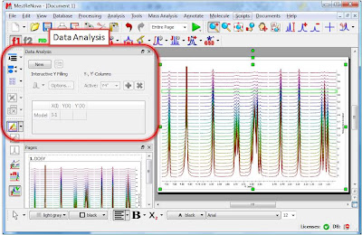
Once the arrayed spectra has been loaded into Mnova, issue menu command Analysis/Data Analysis. The so-called Data Analysis widget will popup. This will be the central control panel (see figure below) for anything related to the analysis of arrayed experiments.

Its operation is very simple. The first thing you have to do is click on the New button. As a result, Mnova will populate the X-Y Table with some initial values (as described in a moment) and create a new item, the so-called Data Analysis Plot. This new item will display the values from the X-Y Table which in general are the values extracted from the arrayed spectra, both experimental (Y) and fitted (Y’).

The X-Y Table

This table is composed by one X column, X(I), one or several Y-columns (Y, Y1, Y2, etc) to hold the experimental values extracted from the arrayed spectra and one or several Y’-columns which hold the fitted values of their Y counterpart columns.

X-Column

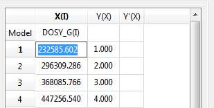
When the table is initialized, in the case of PFG experiments the X-column is populated with the Z values from the Diffusion table, that is, the gradient strengths scaled by taking into account the constants from the selected Tanner-Stejskal model. In the case of a relaxation experiment, the X column will contain the time delays. Of course, it is possible to change the contents of the X-column by following any of these methods:

• Manual editing of the individual cells

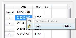
• Copy & paste from a text file. For example, you can put the values for the X-column into a text (ASCII) file and then paste its contents into the table. To do that, just right click on the first cell you want the paste action to start from.

• Enter a formula into the Model cell. Double click on the X(I) model cell (1) and then enter the appropriate equation to populate the X column (2). For example, if you simply enter I, the X column will be filled in with numbers 1, 2,3, etc. If you enter a formula like 10+25*I, the X column will be filled with numbers 35,60, 85, etc.

Y-Column

In all cases, when the table is initialized, the Y-column is automatically filled in with values 1,2,3, etc. The purpose of this column is to hold the experimental values from the arrayed experiment. For example, in the case of a PFG experiment, it may contain how the intensity (or integral) of a given peak (or set of peaks) evolves as the applied pulse field gradient changes. Likewise, in the case of T1/T2 experiments, this column will show the relaxation profile of a given resonance (or set of resonances). So the question is: how to populate the Y-column with actual information from the spectra?

This is again very easy. There is a graphical way (mouse driven) and a manual one. Let’s start with the graphical method:

• Graphical Selection: Click on the ‘Interactive Y Filling’ button (see red-highlighted button in the image below). After doing this, the cursor will change into an integral shaped cursor expecting you to select the region from where you want the integrals to be extracted across all the subspectra in the arrayed item. After the selection is done (see figure below), all the integrals will be placed in the Y column and those values will be displayed in the X-Y plot as green crosses (note: the shape, color, etc of these crosses can be customized from the X-Y plot properties).

• Manual selection: if you take a closer look at the Data Analysis table in the figure above, you can appreciate that once the integral region has been selected, the program shows the following text: Integral(4.752, 4.907). This means that we have selected an integral covering that range. This value can be edited manually so that you can specify the limits by simply editing that cell.

Y’-Column

The Y’ column is reserved for the fitted values assuming a particular theoretical model (e.g. a exponential decay). In this particular case, as we are dealing with PFG experiments, we will be interested in the calculation of the Diffusion coefficients and thus, our fitting model could be a mono-exponential decay (multi-exponential decays can also be handled with this module, but I will not address this problem in this post). The process is very simple:

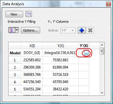
First click on the Y’(X) cell and then on the small button with 3 points as indicated in the figure below.

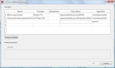
This will launch a dialog box with powerful fitting capabilities.

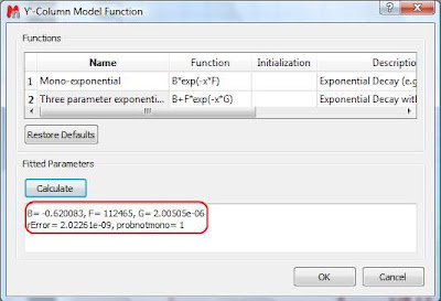
This dialog provides two predefined functions useful for fitting mono-exponential data (such as PFG and Relaxation NMR experiments) using either a 2- or a 3-parameter fit. Furthermore, this dialog offers the possibility to enter user customized functions. As this post is already taking too much space, I will leave the details on data fitting for the next post. For the time being, suffice to say that if your problem regards mono-exponential functions, just select any of the 2 predefined functions in the dialog box and click on the Calculate button. Mnova will immediately compute the optimal values, returning these optimal values as well as the fitting error) and the probability that the acquired series follows the chosen monoexponential model.

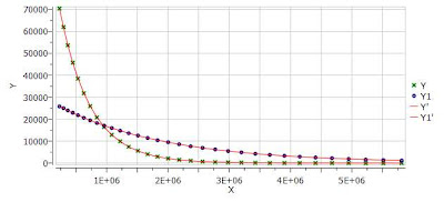
Finally, after closing the dialog, it will populate the Y’ column and the X-Y will be updated with the fitted curve (Red line in the figure below).

One nice feature of the Data Analysis module is its ability to handle multiple series. For example, it’s possible to analyze the decay of several resonances within the same experiment. In order to do that, just click on the (+) button to add a new series and repeat the same process to select the desired resonance range and fit the values. For example, in the figure below I’m showing two curves with different decay rates.

In my next post I will cover some more details about the different methods available to select the intensities/integrals from the spectra and some basic points on the fitting algorithm.
BTW, you can download the full PFG data set used in this post

Basics on Arrayed-NMR Data Analysis (Part II): Practical hints

Further to my previous post, I will cover today some more basic tools available in Mnova for the analysis of NMR arrayed experiments. In particular, I will touch on the following points:

• How to use different display modes for 1D arrayed spectra
• How to navigate throughout the different subspectra in the arrayed item
• How to process individual spectra separately

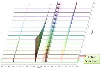
When an arrayed experiment has been detected, all subspectra are grouped together and plotted in the stacked display mode in Mnova (see figure below). Several points are worth mentioning:

(A). Take a look at the green box in the figure below: it shows the so-called ‘active spectrum’. What does this mean?

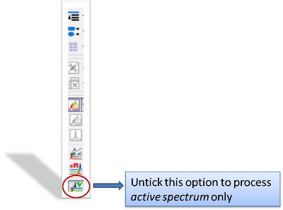
The concept of active spectrum is easier to illustrate with the following example: as I wrote in my previous post, in general all the spectra in an arrayed item are processed exactly with the same processing operations. For example, same level of zero filling, same apodization function, same FT type, same phase correction, etc. However, it i’s possible that some particular spectra require a slightly different processing, independently from the others. In order to do that, it i’s necessary to deactivate the ‘Apply Processing to All spectra in Stack’ option.

So if that option is off, any processing operation will be applied only to the active spectrum in the stack.

The question is: how can we change the active spectrum? There are 3 different ways:

1. Just click on the spectrum you want to be active. This is probably the most intuitive way.
2. Use SHIFT + Mouse Wheel to navigate throughout all the spectra in the stack, one after the other.
3. Use SHIFT + Up/Down arrow keys. This is analogous to point 2)

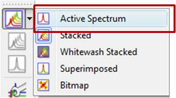
(B). If the number of subspectra (traces) is large (e.g. > 10), working in the stack mode might not be very practical. Quite often, working only with the active spectrum on the screen will be a much better option. This mode can be activated as shown in the image below.

While working on this mode, you will see on the screen just the active spectrum. Should you want to move to another spectrum without resorting to the stack mode, just use methods 2) and 3) described above (Shift+Mouse Wheel or Shift + Up/Down keys).

IMPORTANT: Remember that even if only the active spectrum is visible, unless the “Apply Processing to All spectra in Stack” option is off, all spectra in the stack will also be processed.

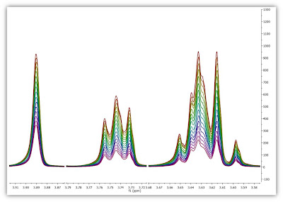
(C) Another useful display mode consists of superimposing all subspectra (see figure below). This method is very useful, for example, when you want to check whether some peaks shift their position (for instance, due to differences in pH, temperature, etc., as is common in biofluids spectra).

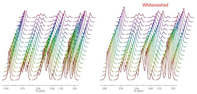
Finally, there is an additional display mode, the so called whitewashed stacked plot. The whitewashing effect means that the spectra at the front of the display hide the spectra behind them from view, as depicted in the figure below.

This plotting mode can be useful to create nice reports, but it’s important to emphasize that drawing time will be significantly higher than with the other plotting modes, so it is not recommended when processing the spectra in real time (e.g. interactive phase correction).

In my next post I will show how to extract useful information from arrayed spectra.

Basics on Arrayed-NMR Data Analysis (part I)

In this post I will cover some basic concepts on the analysis of a very important class of NMR experiments, the so-called Arrayed NMR spectra. The concept is very simple: an arrayed experiment is basically a set of individual spectra acquired sequentially and related to each other through the variation of one or more parameters and finally grouped together to constitute a composite experiment. These experiments are also known as ‘pseudo-2D’. For example, in the case of Bruker spectra they have the same file name as 2D spectra, that is ser files (ser = serial spectra) . In the case of Varian, the file name is fid (Varian uses the same name for 1D, 2D, 3D, … and arrayed spectra). However, unlike with actual 2D spectra, arrayed spectra are only transformed along the F2 –horizontal or direct- dimension (assuming 1D arrayed spectra only).

The modus operandi is better explained with an example: let’s suppose it is necessary to acquire a pulse field gradient (PFG) experiment. Instead of acquiring independent spectra, it is more convenient to create an array with increasing PFG amplitudes. All resulting spectra are now treated as a single experiment. This grouping greatly facilitates processing as, in general, all subspectra require the same processing operations (apart from some occasional minor adjustments of one or several spectra). More about this in a moment.

Well known examples of NMR arrayed experiments are, among others:

• Relaxation (T1, T2)
• PFG experiments (DOSY)
• Kinetics and reaction monitoring by NMR

Any good NMR processing software should be able to automatically recognize when an NMR spectrum is an arrayed experiment and will setup all processing operations accordingly. For example, the figure below illustrates the results obtained when a Bruker arrayed folder is dragged and dropped into Mnova:

What has happened here are basically 2 things:

1. First, Mnova detects that the dropped folder contains an arrayed experiment
2. With that knowledge in hand, Mnova proceeds to process all the individual spectra, one after the other and of course, along the only valid dimension (F2). So for every spectrum, Mnova applies appropriate weighting, zero filling, FT, phase correction, etc and stacks all the spectra as shown in the picture above

As a result, all individual spectra grouped within one composite item (i.e. arrayed item) have been processed in the same way. However, it’s very common that some subspectra might require independent tuning. For example, many PFG NMR experiments present gradient dependent phase shift so that it becomes necessary to adjust the phase of some individual spectra separately. This is very easy to accomplish with Mnova and it will be the subject of my next post.

Mnova 6.0, at last! GSD, Line Fitting, Data Analysis, handling of LC/GC/MS data and much more!

It's been over 6 weeks since my last post on this blog but don’t worry, I haven’t been idle. On the contrary, I have a very good excuse for this lack of posts: We all at Mestrelab have been working very hard trying to get version 6.0 of Mnova finished. Now I’m delighted to announce that we have done it and version 6.0 is finally available for download from our Web site. This is certainly a major upgrade of the software in which we have put a lot of work and passion. It brings a number of enhancements and bug fixes but most significantly are the following new developments:

Mnova MS

Yes, Mnova speaks a new language now, not just NMR. Since its conception, Mnova was Multi-document, Multi-Page, Multi-Platform and designed to become Multi-Technique, which it has now done

GSD (Global Spectral Deconvolution)

I have already blogged about it, but now GSD is finally available so that you all can try it and play with it. We are confident that this new powerful analysis tool will open new avenues in many NMR fields

NMR Line Fitting (Deconvolution)

Even though GSD is a fully automatic spectral deconvolution algorithm, a general purpose line fitting (deconvolution) module is always useful. In an effort to maximize user experience, we have developed a powerful, yet easy to use Graphical User Interface which makes possible both the manual and automatic adjustment of any peaks parameters (i.e. peaks positions, heights, line widths, shapes). I will talk more about it in a new post in a few days


NMR Data Analysis Module

Designed for the analysis of arrayed NMR experiments such as DOSY, Relaxation (T1, T2), kinetics, metabonomics, reaction monitoring, etc. This new module includes, among other features, the capability to apply reliable and fast non linear fitting (including specialized mono-exponential fitting), plotting of the experimental and fitted data, etc

Well, this list is not a fair account of all the number of new things implemented in this version. For a detailed list you could check out the ‘What’s new in 6.0'.

From here I encourage you to try this new version and experiment with the new tools. You can download an evaluation version from our website (at www.mestrelab.com). If for some reason your license has already expired, please do not hesitate to get in touch with us at Mestrelab, we will be delighted to supply a license for the software. In the meantime, I can only add that in the next few days I will be creating new posts where I will be revealing in detail each and every new tool of this brand new version as well as some innovative and interesting applications

Agilent Technologies to Acquire Varian

This morning I got up with this shocking news:
Agilent Technologies to Acquire Varian, Inc. for $1.5 Billion
http://www.agilent.com/about/newsroom/presrel/2009/27jul-gp09016.html

Note:
Just to clarify, the word shocking was used in the sense of surprising, and with no negative connotations meant. Not being privy to the detail of the deal or to Agilent's plans, I can of course not foresee how this may affect Varian's position in the NMR marketplace or how it may affect the NMR community, although having a big company with a big interest in R&D like Agilent in our market could well be very positive

Fighting against peak overlap – Introducing Global Spectral Deconvolution (GSD)

1H NMR is for sure the most powerful technique for structure elucidation, especially for small organic molecules. Typically, an organic chemist uses the chemical shift, coupling constants and integration information contained in an 1H-NMR spectrum to either verify or elucidate an unknown compound. Of course, it’s quite common that a simple 1H-NMR spectrum is not enough to unambiguously confirm a structure and thus other NMR experiments (e.g. 13C-NMR, HSQC, COSY, etc) are used to get more structural information.

Nevertheless, I have often found that many organic chemists do not always try to get the most out of 1H-NMR spectra (which is the cheapest experiment), in particular when some multiplets are complex to interpret (strong coupling) or when peaks overlap prevents valuable information to be detected in some multiplets. Overlapping peaks and new ways to get around it will be the subject of this post.

As it is well known, there are two principal factors limiting the resolution power in a spectrum. First, we have the natural line width limitation imposed by the T2 (spin-spin relaxation). For example, if T2 is about 1 second, the peak linewidth at half height cannot be less than 0.32 Hz (remember, line width at half height = 1 / (pi * T2) = 1 / 3.1415 = 0.32) no matter how powerful is our NMR instrument or the field homogeneity. On the other hand, there are instrumental shortcomings (e.g. spatial uniformity of the applied magnetic field, etc).
Nonetheless, there is an additional limiting factor, and whose importance is generally underestimated which has to do with the generally large number of transitions in 1H-NMR spectra. In short, the peaks we can observe in a 1H-NMR are just a small fraction of the actual transition resonances which are not observable because of the limited digital resolution. In fact, every peak in an 1H-NMR spectrum is basically an envelope of a large number of transitions and its shape is dominated by the coupling pattern of the spin system. Even in molecules of modest size the number of distinct peaks is tens to thousands times smaller than that of quantum transitions. As a very simple example, consider an A3B2 spin system. Depending on the second order interaction and on the available digital resolution, we might observe the expected triplet / quadruplet multiplet patterns. This is illustrated in the figure below.



However, if we use Mnova capabilities to display all main transitions of any coupled spin system by simply hovering with the mouse over the particle of interest, we can appreciate the additional number of resonances (see below):


Furthermore, I can easily increase the digital resolution of the A3B2 spectrum above by just reducing the line width used in the spin simulation module of Mnova. As a result, it’s now possible to observe more resonances in this particular A3B2 spin system (although not all of them, of course):


Of course, this way of increasing the digital resolution is only possible with synthetic spectra and cannot be applied to experimental data. Obviously there are many resolution enhancement techniques being Resolution Booster one of the most powerful ones. As a nice example of the application of this technique, let me tell you this story:
A couple of weeks ago, a very good friend of mine, a professor of organic chemist, came to me with an interesting structural problem. His research group had carried out a reaction which resulted in one single product whose 1H-NMR spectrum was, in principle, compatible with two potential structures. In order to ambiguously find the right structure, they acquired more NMR spectra (DEPT, HSQC, HMBC, COSY) which allowed them to find the correct molecule However, while discussing the problem having a few beers at a bar in Santiago, we found that just the 1H spectrum was more than enough in order to discard one of the two structures and completely assign the correct one without the necessity to acquire any other NMR experiment. The key was the ability to resolve a long range coupling (homo-allylic) with the assistance of Resolution Booster. Basically, the 1H-NMR showed a clean double doublet which was compatible with both structures (I’m sorry, but I cannot reveal those structures). This multiplet is shown below:


After appling Resolution Booster, we could clearly appreciate a further splitting which we could assign to the expected homo-allylic coupling with a value of 1.76 Hz. This coupling was also found in its corresponding multiplet partner confirming the structure:


At this point, it’s worth mentioning that Resolution Booster is a very powerful method to resolve overlapped peaks, but it cannot be used for integration as the area of the peaks get distorted by this process. The good news is that we have developed a new method which in addition to taking advantage of the power of resolution booster, it yields accurate integrals.

This method has been named as Global Spectral Deconvolution (GSD) and as its name says, it automatically deconvolves all the peaks in a spectrum. In short, this method first recognizes all significant peaks in a spectrum, then assigns a realistic a-priori bounds to all peak parameters (chemical shift, heights, line widths, etc) and finally fits all these parameters in a very reasonable time.
Following with the example above, if we apply GSD, we get a multiplet with all the individual peaks clearly resolved and this time, with accurate integrals.


It’s important to mention that we haven’t just fitted the multiplet above, but we have actually fitted the whole spectrum!



We are confident that GSD will open new avenues in NMR data interpretation and quantitative analysis (qNMR). I will blog about these points in future posts.