Now that ENC is practically around the corner, here is a link that shows how far this conference encourages the participants’ creativity:
Pulse Sequence Blues!
NMR can also be fun :-)

Wednesday, 23 February 2011
Thursday, 10 February 2011
Alignment of NMR spectra – Part VI: Reaction Monitoring (II)
Previous posts on this series:
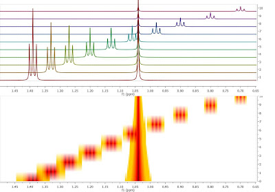
Crossing over of peaks is a very common event in Reaction Monitoring (RM) experiments. When this happens, the automatic alignment algorithm discussed in previous posts (here and here) might not work properly. To illustrate this issue, as I did not have a real experiment at hand, I simulated using Mnova a very simple data set comprised by a triplet and a singlet in such a way that the chemical shift of the triplet moves from 1.4 ppm to 0.7 ppm and having an exponential decay from spectrum to spectrum. This is depicted in the figure below, both as a stacked and a bitmap plot.
Crossing over of peaks is a very common event in Reaction Monitoring (RM) experiments. When this happens, the automatic alignment algorithm discussed in previous posts (here and here) might not work properly. To illustrate this issue, as I did not have a real experiment at hand, I simulated using Mnova a very simple data set comprised by a triplet and a singlet in such a way that the chemical shift of the triplet moves from 1.4 ppm to 0.7 ppm and having an exponential decay from spectrum to spectrum. This is depicted in the figure below, both as a stacked and a bitmap plot.

Now let’s say you are interested in extracting the intensities of the triplet as the reaction progresses. There is actually no need to pre-align the spectra algorithmically; it is much simpler to have some kind of graphical tool to instruct the software which peaks (or multiplets) need to be used for the reaction monitoring analysis. Let me show you how this works in Mnova:
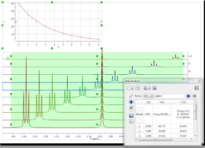
First of all, in the Data Analysis module you select the region to be analyzed. As a starting point, the region will have a rectangular shape (green rectangle in the figure below):

It can be noted that the graph shows an exponential decay, but the actual values must obviously be wrong as the values calculated, using the green rectangle as a boundary for the integration, include peaks from both the triplet and singlet, and we are interested in the analysis of the triplet resonances only. Now let’s change this…
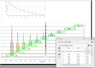
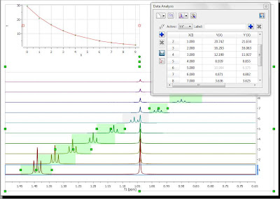
The selection rectangle has a number of handlers (small green boxes). You can drag and move them freely so that you can adjust the selection feature to follow the triplet (BTW, the number of handlers can be adjusted. In this case, there are 6 handlers, but higher numbers are also permitted). In the figure below, the result of adjusting the handlers to follow the triplet is shown:

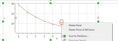
Now you can see that there is an outlier in the exponential curve which, obviously is caused by the singlet which overlaps with the triplet (spectrum number 6 which corresponds to data point #5, as in the graph the numbering starts from zero). Figure below shows that particular spectrum showing the singlet overlapping with the triplet:

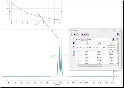
At this stage, there are several approaches. The simplest one is to just discard that point for the analysis, for example, by right clicking on that point in the graph and disabling it:

As soon as that point is deleted / disabled, Mnova will update the graph automatically. This is the new result:

Another approach would involve using GSD to eliminate the singlet from the triplet so that it would not be necessary to discard the information from that particular spectrum. However, this is something I will blog about in a future post.
Tuesday, 8 February 2011
Alignment of NMR spectra – Part V: Reaction Monitoring (I)
Previous posts on this series:
1. Alignment of NMR spectra – Part I: The problem
2. Alignment of NMR spectra – Part II: Binning / Bucketing
3. Alignment of NMR spectra – Part III: Global Alignment
4. Alignment of NMR spectra – Part IV: Advanced Alignment
Following the progression of chemical reactions by NMR is becoming more and more popular. Quoting Michael A. Bernstein et al. (Magn. Reson. Chem. 2007; 45: 564–571)
(…)The technique is rich in structural information, and can uniquely provide subtle information on speciation, protonation sites, and intermediate compound production. NMR measurements can be made under quantitative conditions, and one can be confident that all organic species will be observed. These factors combine to make NMR a very attractive tool for these analyses, and address many of the shortcomings in traditional spectroscopic measurements (…)
Typically, as a reaction proceeds, it’s very common to observe very significant chemical shift fluctuations of a given resonance due to, for example, changes in pH or protonation of the starting material, just to mention a few. These changes in chemical shift can be so large that extracting relevant information from those spectra (e.g. intensities/integrals across the data set) can be difficult, so aligning those spectra can be helpful. Let me illustrate this with an example exhibiting clear nonlinear misalignments: peaks at about ca 11.6 ppm do not move whilst the peaks at higher field move very significantly:

Instead of displaying the data set as a stacked plot as above, it might be more convenient to display it as an intensity or bitmap plot because this plotting mode highlights more clearly the alignment /misalignment profiles:

It’s evident that correcting the data using a single reference peak (or a global shift) is not sufficient. In order to align this data set, we can follow two different strategies:
Strategy 1:
Starting with raw spectrum (1), it is possible to perform a full-spectrum correction (global alignment) before the single intervals are aligned:

It can be appreciated that after applying the global alignment, most of the peaks in (2) are now properly aligned, except the peaks at the left which were previously aligned but after this operation get misaligned. This problem will be covered in the next step.
After the spectra have been aligned ‘globally’, the user just needs to select the interval which comprises the peaks left to be aligned as depicted in (1). (2) shows the final result once both the global and local alignment have been applied:

Strategy 2:
A different, although analogous strategy, would consist in aligning two different spectral intervals separately without resorting to a global alignment as shown in (1) below. Note that the peaks in the interval in the left are already well aligned (so selecting this region is optional; if there were some minor misalignment, the algorithm would optimize such residual misalignment).

(2) shows the final result after the two intervals have been aligned. It’s completely equivalent to the result obtained with Strategy 1
Conclusion
In this post I showed how the automatic alignment algorithm can be used to align RM data sets prior to any further analysis. However, there is a better way to extract NMR descriptors from Reaction Monitoring experiments that does not require any prior pre-processing alignment. In fact, I believe that this method, which I will present in my next post, has several advantages (in the context of reaction monitoring), especially in those cases where the chemical shift ordering of some peaks changes during the reaction, situations in which automatic alignment algorithms usually have great trouble dealing with. An example of a reaction monitoring data set showing peaks crossing over is shown below, in bitmap mode (it’s a simulated data set)

Therefore in my next post, I will show how to analyze RM data sets with important peak fluctuations and crossing over
Monday, 7 February 2011
Alignment of NMR spectra – Part IV: Advanced Alignment
Previous posts on this series:
As I mentioned in my previous post, simple alignment based on shifting or referencing the whole spectrum is not enough in cases where there are different local chemical shift fluctuations.
Resorting back to the synthetic data set used in the previous posts, let me introduce a semi-automatic method designed specifically to align spectra having local chemical shift variations. From a practical point of view, the User needs to select the spectral regions to be aligned and then the program will automatically align those regions separately by using the same technique showed in my last post, that is, maximization of the cross-correlation function. The picture below shows the spectrum before alignment and the two selected regions (top) and the result obtained after applying the alignment algorithm (bottom).

Before going into the details of the automatic alignment algorithm, there is a point I think is worth mentioning: when you have several spectra to be aligned, it is necessary to specify the spectrum which will act as the reference (alignment target). Our implementation provides the capability to use as a reference any spectrum in the data set or the average spectrum.
Automatic Alignment: What is under the hood
Assuming that the spectral segments to be aligned are represented by two vectors g and h, a new vector f can then be generated by cross-correlation:

where * indicates the complex conjugate.
The cross-correlation implemented in Mnova is computed using the fast Fourier transform (FFT), which is a fast O(N log2[N]) process. Briefly, the strategy is to perform an FFT on each of the two vectors, invert the sign of the imaginary part of one Fourier domain representation of one of the vectors, multiply the two Fourier domain functions, and transform the result back using the inverse FFT. By simply calculating the index corresponding to the maximum of f(n) one can find the number of points in which vector g has to be shifted in order to get the highest cross-correlation with respect to h.
This is not, of course, the first time that cross-correlation has been applied for the alignment of two (or more) vectors. Actually, it has been extensively used for alignment purposes in many different contexts, including:
Very recently, we have improved the traditional cross-correlation algorithm by working on the first derivative domain calculated using an improved Savtizky-Golay routine in which the order of the smoothing polynomial is automatically calculated. The idea is to minimize potential problems caused by baseline distortions or very broad peaks.
We have found this method to be very useful not only in the context of metabonomics, but also in the alignment of Reaction Monitoring data sets. However, I better leave this topic for my next post …
- Alignment of NMR spectra – Part I: The problem
- Alignment of NMR spectra – Part II: Binning / Bucketing
- Alignment of NMR spectra – Part III: Global Alignment
As I mentioned in my previous post, simple alignment based on shifting or referencing the whole spectrum is not enough in cases where there are different local chemical shift fluctuations.
Resorting back to the synthetic data set used in the previous posts, let me introduce a semi-automatic method designed specifically to align spectra having local chemical shift variations. From a practical point of view, the User needs to select the spectral regions to be aligned and then the program will automatically align those regions separately by using the same technique showed in my last post, that is, maximization of the cross-correlation function. The picture below shows the spectrum before alignment and the two selected regions (top) and the result obtained after applying the alignment algorithm (bottom).

Before going into the details of the automatic alignment algorithm, there is a point I think is worth mentioning: when you have several spectra to be aligned, it is necessary to specify the spectrum which will act as the reference (alignment target). Our implementation provides the capability to use as a reference any spectrum in the data set or the average spectrum.
Automatic Alignment: What is under the hood
Assuming that the spectral segments to be aligned are represented by two vectors g and h, a new vector f can then be generated by cross-correlation:

where * indicates the complex conjugate.
The cross-correlation implemented in Mnova is computed using the fast Fourier transform (FFT), which is a fast O(N log2[N]) process. Briefly, the strategy is to perform an FFT on each of the two vectors, invert the sign of the imaginary part of one Fourier domain representation of one of the vectors, multiply the two Fourier domain functions, and transform the result back using the inverse FFT. By simply calculating the index corresponding to the maximum of f(n) one can find the number of points in which vector g has to be shifted in order to get the highest cross-correlation with respect to h.
This is not, of course, the first time that cross-correlation has been applied for the alignment of two (or more) vectors. Actually, it has been extensively used for alignment purposes in many different contexts, including:
- Chromatography (Anal. Chem. 2005, 77, 5655-5661)
- NMR (J. Magn. Reson. 2010, 202, 190-202)
- DNA Sequence Alignment (J. Biomol. Tech. 2005, 16, 453–458)
Very recently, we have improved the traditional cross-correlation algorithm by working on the first derivative domain calculated using an improved Savtizky-Golay routine in which the order of the smoothing polynomial is automatically calculated. The idea is to minimize potential problems caused by baseline distortions or very broad peaks.
We have found this method to be very useful not only in the context of metabonomics, but also in the alignment of Reaction Monitoring data sets. However, I better leave this topic for my next post …
Thursday, 3 February 2011
Alignment of NMR spectra – Part III: Global Alignment
Previous posts on this series:
We have seen that binning helps in minimizing, for example, the effect of pH-induced fluctuations in chemical shift so that, in the field of NMR-based metabonomics studies, ensuring that signals for a given metabolite appear at the same location in all spectra. One evident disadvantage of binning is that it greatly reduces the spectral resolution (e.g. in a 500 MHz instrument, a typical 64 Kb NMR spectrum with SW = 12 ppm, would be reduced to 300 points (bins) if a bin width of 0.04 ppm [20 Hz = ~218 points] is used).
This loss of resolution is not desirable and considering that today’s powerful computers can handle large data matrices, there is now an increasing tendency to perform multivariate analysis at the maximum spectral resolution possible. Alternatives to binning typically involve some form of peak alignment procedure and in this post I will cover the simplest one, global alignment. The purpose of this post is to simply illustrate the concept of alignment, but it is important to note that this method is not generally applicable to the misalignment problems found in metabonomics NMR data sets, although it might be useful in many other contexts.
The idea of global alignment is very simple and corresponds to the well-known chemical shift referencing method in which the user sets the internal reference peak (e.g. TMS, DSS, TSP, etc) of each spectrum to e.g. 0 ppm. In order to cope with small fluctuations in chemical shifts, this method seeks for the highest peak within a narrow (user-defined, auto-tuning option in Mnova) interval, as depicted in the figure below:

Clearly, this method will not work properly in those data sets with local misalignments, that is, when signals of one metabolite fluctuates in one direction whilst the peaks of a different metabolite move differently). As an example, let’s consider again the simulated data set of Taurine used in my previous post and which I copy below for convenience:

Remember that this data set has been generated by randomly changing the chemical shifts of the two CH2 groups. Now, let’s apply the global alignment procedure using as chemical shift reference at a value of 3.25 ppm as shown in the picture below:

As expected, all peaks corresponding to the triplet at 3.25 get perfectly aligned, but the other multiplet remains misaligned (see below).

One could devise an extension to this global alignment procedure in which the same procedure is applied to different segments of the spectrum. In this particular case, one could select two different windows, one for each triplet and apply the same algorithm locally to each segment. However, having to manually select the chemical shift reference for each segment is not very practical and, in addition, relying only on the simple search of the maximum peak within each segment is not a very robust method for automatic alignment. In my next post, I will present a much more powerful automatic alignment method in which the user will not need to define the reference chemical shift value for each segment / window, but before that, and as an introduction to that post, let me show you another global automatic alignment method.
Let’s assume that we have several spectra which we want to align automatically in such a way that we first manually reference the chemical shift of one of these spectra (e.g. the first one in the series) and then ask the software (e.g. Mnova) to automatically align all the other spectra using this one as a reference spectrum. The idea for such algorithm is to figure out which is the optimal value that a spectrum has to be shifted (left or right) so that the difference between this spectrum and the reference one is minimal.

Such alternative ‘global method’ has been implemented in Mnova several years ago already and is based on the maximization of the cross-correlation between the reference spectrum and the spectrum/spectra to be aligned. This procedure is the essential foundation for the advanced alignment method which I will present in my next post.
- Alignment of NMR spectra – Part I: The problem
- Alignment of NMR spectra – Part II: Binning / Bucketing
We have seen that binning helps in minimizing, for example, the effect of pH-induced fluctuations in chemical shift so that, in the field of NMR-based metabonomics studies, ensuring that signals for a given metabolite appear at the same location in all spectra. One evident disadvantage of binning is that it greatly reduces the spectral resolution (e.g. in a 500 MHz instrument, a typical 64 Kb NMR spectrum with SW = 12 ppm, would be reduced to 300 points (bins) if a bin width of 0.04 ppm [20 Hz = ~218 points] is used).
This loss of resolution is not desirable and considering that today’s powerful computers can handle large data matrices, there is now an increasing tendency to perform multivariate analysis at the maximum spectral resolution possible. Alternatives to binning typically involve some form of peak alignment procedure and in this post I will cover the simplest one, global alignment. The purpose of this post is to simply illustrate the concept of alignment, but it is important to note that this method is not generally applicable to the misalignment problems found in metabonomics NMR data sets, although it might be useful in many other contexts.
The idea of global alignment is very simple and corresponds to the well-known chemical shift referencing method in which the user sets the internal reference peak (e.g. TMS, DSS, TSP, etc) of each spectrum to e.g. 0 ppm. In order to cope with small fluctuations in chemical shifts, this method seeks for the highest peak within a narrow (user-defined, auto-tuning option in Mnova) interval, as depicted in the figure below:

Clearly, this method will not work properly in those data sets with local misalignments, that is, when signals of one metabolite fluctuates in one direction whilst the peaks of a different metabolite move differently). As an example, let’s consider again the simulated data set of Taurine used in my previous post and which I copy below for convenience:

Remember that this data set has been generated by randomly changing the chemical shifts of the two CH2 groups. Now, let’s apply the global alignment procedure using as chemical shift reference at a value of 3.25 ppm as shown in the picture below:

As expected, all peaks corresponding to the triplet at 3.25 get perfectly aligned, but the other multiplet remains misaligned (see below).

One could devise an extension to this global alignment procedure in which the same procedure is applied to different segments of the spectrum. In this particular case, one could select two different windows, one for each triplet and apply the same algorithm locally to each segment. However, having to manually select the chemical shift reference for each segment is not very practical and, in addition, relying only on the simple search of the maximum peak within each segment is not a very robust method for automatic alignment. In my next post, I will present a much more powerful automatic alignment method in which the user will not need to define the reference chemical shift value for each segment / window, but before that, and as an introduction to that post, let me show you another global automatic alignment method.
Let’s assume that we have several spectra which we want to align automatically in such a way that we first manually reference the chemical shift of one of these spectra (e.g. the first one in the series) and then ask the software (e.g. Mnova) to automatically align all the other spectra using this one as a reference spectrum. The idea for such algorithm is to figure out which is the optimal value that a spectrum has to be shifted (left or right) so that the difference between this spectrum and the reference one is minimal.

Such alternative ‘global method’ has been implemented in Mnova several years ago already and is based on the maximization of the cross-correlation between the reference spectrum and the spectrum/spectra to be aligned. This procedure is the essential foundation for the advanced alignment method which I will present in my next post.
Subscribe to:
Posts (Atom)