Quadruplet, triplet … so simple?

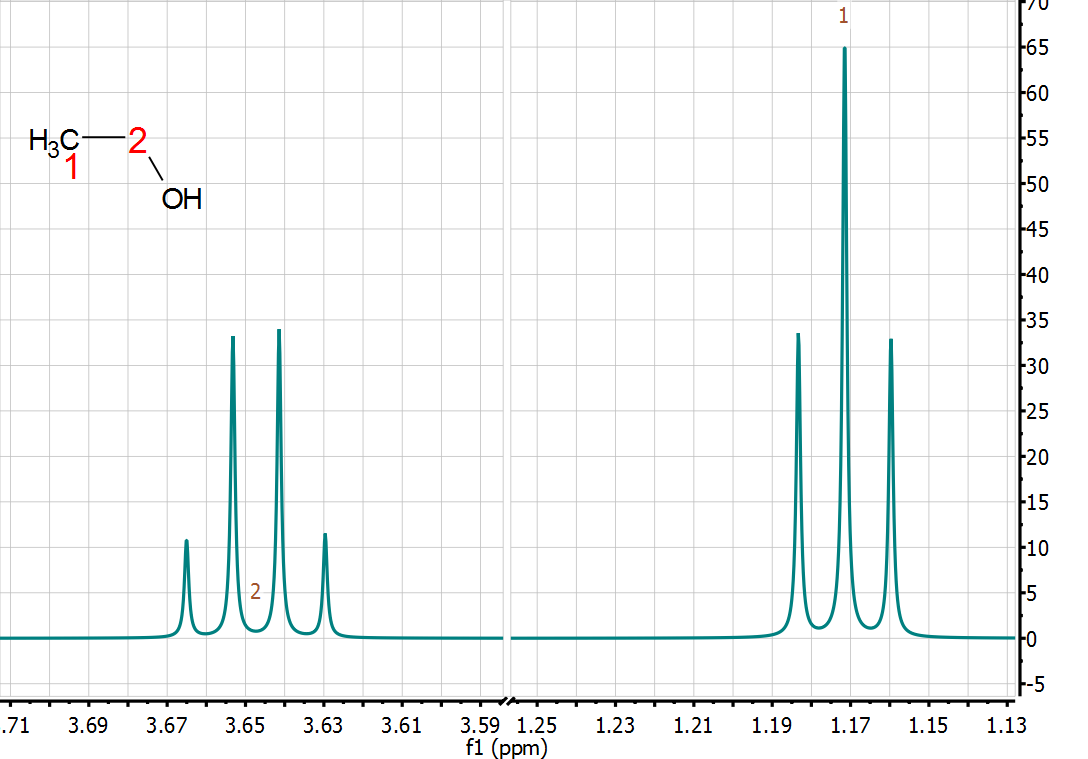
In the picture below I’m showing the ‘synthetic’ NMR spectrum of Ethanol. It has been synthesized using Mnova Spin Simulation capabilities and the experimental values (chemical shifts and couplings) taken from the NMR spectrum of ethanol recorded at 600 MHz in water, so the OH signal will not show up.

Nothing new under the sun. This is a very simple spectrum where the two observed multiplets seem to follow very nicely the well-known first order multiplet rules that most chemists use on daily basis. In this case, a very simple A3X2 spin system.

But does this mean that this spectrum is actually composed by only 7 peaks? The answer is, of course not, there are many more peaks! But because of the very limited resolution, most of them are not observed and merge in such a way that only 7 peaks are ultimately observed.

In other words, the number of NMR transitions is usually much larger than the number of peaks we actually observe in the spectrum. Just to give an example: A molecule containing 30 coupled protons will result in a spectrum having 16106127360 (=1.61E+10) transitions. As its corresponding NMR spectrum will show only about 100-200 peaks, that makes it well over eighty million quantum transitions per resolved peak!

For example, let’s magnify the quadruplet and use Mnova unique capabilities to display the individual transitions by simply hovering with the mouse cursor over the atoms in the molecule (CH2 in this case). We can see that there are some ‘hidden peaks’, these are the NMR transitions calculated by diagonalizing the NMR Hamiltonian.

These transitions are so close that they cannot be resolved under the usual NMR resolution conditions. In fact, to separate all these signals, it would be necessary to have a spectral resolution of < 0.01 Hz

Whilst this is far from being feasible experimentally nowadays, it is easy to do numerically. In the figure below I’m displaying the same synthetic spectrum of Ethanol but this time synthesized using a line width of just 0.01 Hz and 1 MB of digital data points. Now the individual transitions can be seen as resolved peaks so in this example a transition will be virtually equivalent to an NMR peak.   

Simply put, an NMR spectrum is just a superposition of all spectral transitions (which can be in the order of millions), transitions compose peaks, peaks group into multiplets, and multiplets compose the spectrum.

The ability of Mnova to show the individual NMR transitions in a synthetic spectrum can be a good teaching tool

For a more theoretical and rigorous discussion on NMR transitions, see A.D. Bain, D.A. Fletcher and P. Hazendonk. "What is a transition?" Concepts in Magnetic Resonance 10 85- 98 (1998) (link)

From NMR multiplets reports to synthetic spectra

I admit that I was never a fan of the traditional way in which NMR spectra are usually reported in organic chemistry journals, something like:

¹H NMR (300 MHz, CDCl₃) 7.91 (d, J=8.2 Hz, 2H), 7.31 (d, J=8.2 Hz, 2H), 3.65 (t, J=6.3 Hz, 2H), 3.13 (t, J=6.9 Hz, 2H), 2.95 (p, J=6.9 Hz, 1H), 2.20 (p, J=6.6 Hz, 2H), 1.26 (d, J=6.9 Hz, 6H)

It is not only that there is not a standard format that is strictly followed by all journals. It is also that it does not convey all the NMR information contained in the actual spectrum (reducing a spectrum into a multiplet report results in an irreversible loss of important information) and facilitates the job to those willing to cheat ( see this and this).

Today, in the 21st century, I don’t see any reason why the experimental raw data (i.e. FID+metadata) should not be an integral part of any article where NMR spectra have been used to characterize a chemical structure. In any event, there are millions of articles with NMR spectra in the form of those old fashioned multiplet reports and we thought that it would be a good idea to implement some tools to facilitate the analysis of those reduced spectra.

That is why we developed the Mnova script “Multiplet Report to Spectrum”, a tool which is available in Mnova from the scripts menu:

It is very easy to use: Once this command is issued, you only need to copy to the clipboard your multiplet report from the article (PDF, Word document, etc) and paste it into the Multiplet report edit box at the top of the dialog:

As soon as it is pasted, this application will parse the multiplets and the different fields (chemical shifts, number of protons, multiplicity, solvent, nucleus, etc) will be automatically populated. If for any reason some of those values are not correctly parse, you can manually amend them.

Once you are happy with those values, you can press OK so that Mnova will synthesize a spectrum with those values.

We believe that this is a very useful tool, in particular for organic chemists. It can be used to easily compare an experimental spectrum with a multiplet report from a journal, for example.

PCA and NMR: Practical aspects

As of version 9.0, it is possible to perform PCA of NMR data sets directly from within the Mnova User Interface without having to resort to third party applications. The basic PCA functionality has been previously covered in this blog (see Chemometrics under Mnova 9 – PCA) and in this entry we are going to discuss in more detail some more practical aspects, particularly on the different binning, filtering and scaling options. 

What follows has been kindly written by Silvia Mari (project leader of the PCA module) and Isaac Iglesias, who programmed this module in Mnova.

Introduction

Matrix generation from an array of NMR spectra is the core step in chemometric analysis. This procedure involves several options that the user should chose. In this entry we want to focus on the practical aspects concerning matrix preparation from NMR data. Broadly speaking, we can consider three main issues:

1. Choice of binning method: Sum vs Peak
2. Filtering or not filtering?
3. Choice of Scaling strategy

Choice of binning method: Sum vs Peak

When dealing with high resolution NMR spectra it is in general impracticable to work with the entire data points of the spectra which are usually in the order of 32Kb and bigger. The most common strategy used to reduce the number of variables consists in dividing each spectrum in a defined number of regions, the so called bins.  Several binning strategies are available today, from regular binning, where bins have fixed width, to more sophisticated strategies such as gaussian or dynamic adaptive binning [1]. But even for these cases, when dealing with particularly crowded spectra, it usually happens that shifts in peaks close to bin boundaries can cause dramatic quantitative changes in adjacent bins. A good help in solving this problem could come from peak deconvolution strategies.  Generally speaking, a deconvolved peak is a mathematical entity characterized by a chemical shift (frequency), intensity and half-height line width. The integral of a peak can be automatically derived assuming a peak shape (i.e. Lorentzian) and the intensity and line width. For this reason, binning a spectrum of deconvolved peaks reads out virtually completely the problem of bin boundaries as illustrated in figure 1.

 Figure 1 – Binning real peaks versus binning deconvolved peaks

When dealing with an array of NMR spectra, whilst regular binning of a number b of bins over  stacked spectra containing  s spectra will generate a matrix bxs (see figure 2), it is not possible to generate a similar matrix using directly deconvolved peaks (peak list) since the number and position of peaks varies from spectrum to spectrum

Figure 2 – Matrix generation from regular binning or peak list.

To encompass this problem there are two main strategies: (1) provide algorithms for peak alignment over the spectra series, as well as strategies for dealing with missing peaks in order to end up with the same number of peaks and the same peak positions for all the spectra; (2) perform binning over the peak table.

In the PCA module available in Mnova, we adopt the second solution. User can decide whether to use regular binning (Sum) or binning over deconvolved peaks (Peak) from the binning options. An example of better classification is qualitatively represented in figure 3, where score plots are represented for binning using Sum method (panel A) and binning using Peak method (panel B).

Figure 3 – Score plots obtained using same bin width of 0.03ppm; in both cases data were normalized by the sum and pareto scaled. In panel A bins were obtained directly as integration of real spectra; in panel B bins were obtained by binning of the corresponding peak list obtained after global spectral deconvolution.

Filtering or not filtering?

When reducing bin width to approximate spectral resolution, and hence increasing the number of variables, it is generally required to introduce filtering strategies in order to filter out those variables that do not show significantly changes. There are established filtering strategies that are commonly applied to genomics type of data and that could also be successfully used for NMR-based type of data[1].  In the PCA module we have implemented five filtering options, namely: 

1. Standard Deviation
2. Median Absolute Deviation
3. Interquartile Range
4. Mean Value
5. Median Value 

In the first three cases a fixed fraction (default 10%) of the bins is discarded (e.g. if the matrix is composed by 100 bins it means that 10 bins are discarded) and the selection is based on the Filter method chosen. In the case of Mean Value or Median Value, user is asked to input a value for the Mean or the Median. By doing so, only bins that display a lower value of the inputted one are discarded. In the following figure, the difference in clustering capability when the filtering is applied or not is illustrated. Finally, it worth noting that very often, NMR data can contain regions which should discarded and included into the so called blind regions; these regions will not be taken into account in the principal component calculation.

Figure 4 - Score plots obtained using same bin width of 0.01ppm; in both cases data were normalized by the sum and pareto scaled. In panel A no filter was applied; in panel B filtering strategy based on Mean Value was applied. A cut-off value of 100 was used.

Choice of Scaling strategy

Scaling is an operation that is performed on the variables (columns) of the matrix. Scaling strategy depends from one hand from the biological information we wish to extract, but on the other hand also on the data analysis method chosen (in our case PCA). As a first approach the so-called Centering is generally applied to every analysis. With Centering all bin values fluctuate around zero instead of around the mean of each bin; therefore Centering is a method that adjusts for differences in the offset between high and low abundant compounds. There are several methods available in literature for scaling [3], and generally centering is applied in combination with these methods. Scaling strategies could be divided in two subclasses:  methods that use data dispersion (such as standard deviation) as scaling factor; and methods that use size measure (such as the mean). For the first group Mnova includes Auto, Pareto and  Vast scaling strategies. For the second group Range and Level scaling are available. Generally speaking, when dealing with PCA analysis, the first group is normally preferred. Figure 5 shows score plot differences between PCA that used Pareto scaling (A panel) in comparison with PCA that used Level scaling

Figure 5 - Score plots obtained using same bin width of 0.05 ppm and normalization by the sum. In panel A Pareto scaling was applied; in panel B Level scaling was applied.

Conclusions

We have focused on some very practical aspects when dealing with PCA analysis. But it is always necessary to think about how good was our experimental design. Quoting Stanley Deming [4] in his overview of Chemometrics of 1986: ”Chemometrics is primarily concerned with the acquisition of data and the extraction of useful information from that data” and again:” In a given situation, it is far better to err on the side of too many pieces of experimental data. If too few data are available, one might not be able to make any conclusion, and the whole set of experiments will have been wasted”.

Acknowledgments

We are grateful to Dr. Giovanna Musco and Dr. Jose Garcia-Manteiga for providing dataset for testing purposes.

References

[1] Amber J Hackstadt, Filtering for increased power for microarray data analysis. BMC Bioinformatics 2009, 10:11

[2] Paul E. Anderson, Metabolomics, Volume 7, Issue 2, pp 179-190 (2010)

[3] Robert A van den Berg, Centering, scaling, and transformations: improving the biological information content of metabolomics data. BMC Genomics 2006, 7:142

[4] Stanley N. Deming, Chemometrics:an Overview. CLIN. CHEM. 32/9, 1702-1706 (1986)

Learn NMR FID

Last September, in SMASH 2013, I had the privilege of getting a personal demo from Tim E. Burrow of a cool iPad application he was developing that showed in a very nice way the basics of NMR data processing. This app simulates an FID and shows the effects on the corresponding FT spectrum when different apodization functions, zero filling or other time-domain operations are applied to the FID.

Since that day, I nearly forgot about Learn NMR FID until it was very recently brought to my attention after reading this article in Glenn Facey’s blog.

When I installed this app, I was happy to notice one very nice feature that I had discussed with Tim: The FID can be simulated with two spins (1/2) and add a coupling in such a way that it is possible to see, in an interactive way, the difference between weak (i.e. AX spin system) and strong (i.e. AB spin system) coupling.

I believe this is a great educational tool which I will certainly use in any lecture on NMR processing.  Tim did a great job and I look forward to seeing more cool things from him!

Chemometrics under Mnova 9 - PCA

(Note: This entry has been written by Dr. Silvia Mari, from R4R who has helped us to design and implement this module)

Background: spectroscopy and chemometrics

“For many years, there was the prevailing view that if one needed fancy data analyses, then the experiment was not planned correctly, but now it is recognized that most systems are multivariate in nature and univariate approaches are unlikely to result in optimum solutions.”

      Hopke, P. K. (2003). The evolution of chemometrics. Analytica Chimica Acta, 500(1-2), 365–377]
  
Either we apply analytical chemistry for quality and control or we attempt to a more “system biology” approach for our R&D we do need advanced methods to design experiments, calibrate instruments, and analyze the resulting data. And the “emergence of chemometrics thinking came from the realization that traditional univariate statistics is not sufficient to describe and model chemical experiments”
       Geladi, P. (2003). Chemometrics in spectroscopy . Part 1 . Classical chemometrics, 58, 767–782

With this in mind Mnova 9 now offers to its users a module called PCA which could be found under the main menu “Advanced”. It is the result of our first efforts to include chemometric tools into Mnova and it is meant to give spectroscopist the possibility to interactively work on both stacked spectra and its corresponding statistical plots.

Starting from mid ‘70s where the first paper with chemometrics in the title appeared in 1975 [1], chemometrics has grown up and is now considered a functioning research area in the chemical science. It has expanded widely from its beginnings into a variety of other areas including multivariate calibration, pattern recognition, and mixture resolution and today there are several applications of interest for the NMR spectroscopists [2-5].

PCA module

Principal Component Analysis (PCA) is a procedure which uses orthogonal transformation to convert a set of observations from correlated variables into a set of values of linearly uncorrelated variables (named principal components) [6].

PCA module under Advanced menu is working in two subsequent steps: (1) matrix generation and (2) principal component analysis. The overall workflow can be represented with the following illustration, where general steps available in Mnova are highlighted in blue whilst specific functionalities of this new PCA module are highlighted in yellow.

With the aim to help the spectroscopist to refine and optimize the data matrix to be used for advanced analysis, PCA in Mnova makes it very easy the detection and removal of spectrum outliers, reveal problems in spectral alignment as well as in its phase or baseline. Once the user has properly corrected those regions of interest, the PCA module allows to re-run the analysis, either replacing the previous analysis or creating a new one for comparison.

Interaction with the stacked spectra.

The main effort applied during the design and development could be summarized in one word: SYNCHRONIZATION. PCA plots, PCA tables and stacked plot are always synchronized. By doing so selections of a point in the score plot imply a selection in the stacked plot. 

In the same way, a selection of a point in the loading plots (hence a selection of a variable of the matrix) generate a shadow into the stacked plot according to the bin position and size.

Colors and graphics

When dealing with large dataset, color coding plays a very important role and eventually essential. Even if PCA does not use class definition in its algorithm since it is an unsupervised method, the kind of patterns expected is generally known.

The driving concept here is that colors are assigned on the basis of class belonging. Again, as in the previous section, colors are always synchronized from PCA tables to PCA plots and to stacked spectra as well

Moreover, in the loading plot, the user is allowed to select more than one bin (see flag option in the loading plot table, or multiple selection of table entry using shift or ctrl  key). Visualization of a bin region is obtained with a colored box that is displayed superimposed over the stacked plot. The User can associate different colors to different bins regions

Data filtering and scaling

The results of the analysis depend on the types of filtering and scaling of the matrix that user selects, which therefore must be specified. It can be demonstrated how both factors greatly affect the outcome of the data analysis and thus the rank of the most important variables. PCA module includes several possibilities in terms of data cleaning and scaling.

There is not a general rule in the selection of the type of scaling. For that purposes we recommend the manuscript from van den Berg et. al. [7] which describes extensively how these transformations could improve the information content of the data matrix. Finally, bear in mind that visual inspection and assessment is ultimately one of the most important steps in chemometrics.

Conclusion

We have introduced in Mnova 9 a chemometric module called PCA (Principal Component Analysis). PCA have been shown to be very effective in compressing large volume of noisy correlated data into a subspace of much lower dimension than the original data set. Data pretreatment method is crucial to the outcome of the data analysis. The resulting low dimensional representation of the data set has been shown to be of great utility for analysis or monitoring the system under study, as well as in selecting variables for control or markers of the expected pattern.

The possibility to interactively play with PCA plots and spectra at the same time, and the user friendly interface provided by Mnova will be of great advantages also for spectroscopists that are not familiar with multivariate analysis but would like to learn more and test it.
As has always been for Mnova community, the future of this new first step in chemometrics will be driven by user requirements. For that reason we look forward to get feedback, criticisms, suggestions, comments and lots of requests for future development. So, play with it and have fun at looking at your own datasets from a different perspective!

References

[1] B.R. Kowalski, Chemometrics: views and propositions, J. Chem. Inf. Comp. Sci. 15 (1975) 201–203

[2] Chemometrics in bioreactor monitoring. Lourenço, N. D., Lopes, J. a, Almeida, C. F., Sarraguça, M. C., & Pinheiro, H. M. (2012). Bioreactor monitoring with spectroscopy and chemometrics: a review. Analytical and bioanalytical chemistry, 404(4), 1211–37. doi:10.1007/s00216-012-6073-9

[3] Metabonomics and chemometrics in food science and nutrition. Kuang, H., Li, Z., Peng, C., Liu, L., Xu, L., Zhu, Y., Wang, L., et al. (2012). Metabonomics approaches and the potential application in food safety evaluation. Critical reviews in food science and nutrition, 52(9), 761–74. doi:10.1080/10408398.2010.508345

[4] Pharmaco-metabonomic phenotyping and chemometrics. Robertson, D. G., Reily, M. D., & Baker, J. D. (2007). Metabonomics in Pharmaceutical Discovery and Development, 526–539.

[5] Metabonomics and chemometrics in drug safety and toxicology. Griffin, J. (2004). The potential of metabonomics in drug safety and toxicology. Drug Discovery Today Technologies, 1(3), 285–293. doi:10.1016/j.ddtec.2004.10.011

[6] Principal component analysis, Svante Wold, Kim Esbensen, Paul Geladi. Volume 2, Issues 1–3, August 1987, Pages 37–52

[7] Van den Berg, R. A., Hoefsloot, H. C. J., Westerhuis, J. A., Smilde, A. K., & van der Werf, M. J. (2006). Centering, scaling, and transformations: improving the biological information content of metabolomics data. BMC genomics, 7(1), 142. doi:10.1186/1471-2164-7-142

Chemical Shift, Absolutely!

(Note: This entry has been written by Dr. Mike Bernstein - Thank you, Mike!)

It’s a “given” that for NMR the chemical shift must be reported relative to standard. The most widely used is the 1H signal of tetramethylsilane (TMS) in chloroform, which has an assigned value of exactly zero. This is convention, and we all adhere to it. Correctly referencing 1H NMR spectra is seldom a difficulty, whether we use co-dissolved TMS (or a water-soluble equivalent), or the residual proton signal from the deuterated solvent. Things can get more complex, but this works for the vast majority of us. The chemical shift, d, is defined thus:

Venturing to the “dark side” of NMR – nuclei other than 1H – seldom stretches beyond 13C for most, and a residual solvent signal is very often present that can be used as a secondary chemical shift reference. But beautiful possibilities tempt many of us. Whether you are interested in biomolecular NMR and live and breathe 15N and possibly 31P, or 2H, or an orgametallic chemist with an interest in far more exotic nuclei, each heteronucleus has its charms and challenges. One thing unites NMR of all nuclei: adherence to a convention for chemical shifts. This can be easier said than done, given that some reference materials are difficult to handle, expensive, etc. The chemical shift reference compound for 19F NMR is the banned substance, Freon-11.

Absolute chemical shifts

We get help from a group working under the IUPAC [1] guise for their work in helping us calculate the chemical shift scale for all NMR-active nuclei [2].  That is, they provide us with a standard way to get the chemical shift precisely correct for any and all heteronuclear NMR spectra. That’s amazing - and hugely useful!

So how does it work? Well, it’s quite simple, really. At the heart of the calculation is the absolute frequency of the 1H signal of TMS for your NMR spectrometer hardware (console, probe, etc.) and sample (solvent, temperature, etc.). You need to be able to determine the exact frequency of this reference signal to seven decimal figures, at least. The following equation applies (sometimes expressed as a percentage) and uses a ratio to describe a constant, X (Greek capital Xi):

Making it easy with Mnova

We make heavy use of absolute referencing (AR) in Mnova, with the following available:

• Correctly reference an X-nucleus spectrum when the referenced 1H spectrum is available
• Apply AR to heteronuclear axes in 2D experiments
• Allow users to customise the X  values
• Indirect 1H spectrum referencing using n_TMS  for a specific hardware and solvent (locked)

Referencing heteronuclear spectra

Ensure that you have a document having (a) a correctly referenced 1H NMR spectrum, and (b) one or more –nucleus spectra.

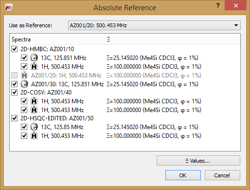
Select Analysis è Reference è Absolute reference… and choose the X-axis spectrum/spectra to reference.  

The table of X values

Note that by tapping on the “X values…” button you will be presented with the table of X-nuclei. In the case of 15N, for example, you can choose which reference standard you want to use. By clicking on the blue “+” button you can enter your own, customised value. 

Referencing 2D spectra

When there are 2D spectra in the document then the Absolute reference… selection will reflect this, and allow you to choose which spectrum is used for referencing purposes, and the traces to which this should be applied. Note that you can adjust the referencing of 1H and X-nuclei.

Referencing a 1H spectrum

You can use saved n_TMS values to reference another 1H spectrum from the same NMR spectrometer. Start with a correctly-referenced 1H NMR spectrum, and select Analysis è Reference è Edit saved references…  From this dialogue you can add the value for the particular hardware and measurement conditions – solvent, temperature, etc. 

Now, when you select Analysis è Reference è Apply saved reference then the saved value will be used if the criteria are met. 

Conclusions

Absolute referencing is a powerful way to ensure that data are correctly referenced. This is equally important in open-access environments as it is under automation, where it helps processes such as Verify be more robust. 

References

[1] (a) Harris RK, Becker ED, Cabral de Menzes SM, Goodfellow R, Granger P. Pure Appl. Chem. 2001; 73: 1795

(b) Harris RK, Becker ED. J. Magn. Reson. 2003; 156: 323.

[2] This is nicely described here: http://www.chem.wisc.edu/~cic/nmr/Guides/Other/Xi_chem_shift_scale.pdf