The bumpy road towards ASV

Figure: Photo taken during our bike climbing to Galibier (Lautaret) in the Tour de France 2011

One of the most exciting and complex challenges in NMR software for small molecules at present is the ability to verify a proposed chemical structure from its NMR spectrum automatically, a process commonly known as Automatic Structure Verification (ASV). Nowadays, it is possible to acquire spectra automatically on large numbers of compounds, but the interpretation of all of this data constitutes a key bottleneck [1]. As John Hollerton wrote in Stan’s blog

So now I come to the purpose of ASV. I don't know of many (any) companies employing people to look at 50 spectra a day (except for specific, one-off projects)

We at Mestrelab have been working for several years already to provide the most powerful and usable ASV software package.

It was not an easy job, and in some ways, resembles the stages of the Tour de France that Santi, some friends and I made a few days ago. We had to suffer, curve by curve, ramp by ramp to reach the top of the mythical Cols of the Alps (Galibier, Alpe D'Huez, Croix de Fer, Telegraph, Les 2 Alpes, etc), but we've made it :-)

Similarly, the road to ASV has also been very steep and tough, but we think now that we have a truly sophisticated and successful system that delivers very good results.

Of course, there's always room for improvement (as with the Alps, which we could climb much faster if we had been riding on road bikes instead of BTTs:-)), but either way, we are very satisfied with the current state of our ASV.

From here I would like to take this opportunity to thank Stan Sykora for his superb work

References:
[1] S.A. Richards, J.C. Hollerton, Essential Practical NMR for Organic Chemistry, John Wiley & Sons, Ltd, 2011.

Intelligent Peak Picking of 1D NMR Spectra

In case you hadn´t noticed, version 7 of Mnova was released just a few days ago.

Whilst this new version presents a number of significant improvements in the software, in this post I would like to focus on a new peak picking concept which, to the best of my knowledge, is novel and in some way, revolutionary. I will try to keep this as short and clear as possible, just to illustrate the very basic ideas that motivated this new approach to peak picking. In the next posts I will elaborate further on some of the new points introduced here.

Traditional Peak Picking

First up, to lay the groundwork for this article, let’s revisit the way in which peak picking algorithms usually work in all NMR software packages, including the former versions of Mnova: Essentially, in this procedure, all peaks maxima (and/or minima) in a spectrum are determined and their values are either stored in a tabular form (i.e. in a peak table) or displayed graphically over the spectrum (Figure 1).

Figure 1: Illustration of traditional peak picking

Each NMR application might offer different levels of sophistication in the peak picking algorithms. For example, some can resolve overlapped peaks better than others (http://nmr-analysis.blogspot.com/2009/06/fighting-against-peak-overlap.html ), others operate more efficiently with spectra with low SNR, etc.), but the important element I would like to highlight here is the fact that the output of any peak picking algorithm is just a plain list of significant points in a spectrum.

So far, so good. The question is: What is the purpose of applying peak picking? Well, there is no definitive answer and it depends upon the particular application. Nonetheless, if we restrict the context to that of the simple analysis of small molecules for their characterization, peak picking is usually applied to the calculation of coupling constants and chemical shifts, (in other words determination of the spin system(s) in the spectrum). Whenever practicable, this should be done as automatically as possible by the NMR Software.

Historically, this automatic analysis was based on Quantum Mechanical (QM) methods [1]. They are certainly the most rigorous yet complex methods, although interestingly, the most popular approaches even more than 40 years ago [2-4] when computer power was much more limited than today.

Another approach, which incidentally has attracted significant interest in recent years, despite being computationally much less demanding, is based on the same technique typically used by organic chemists, i.e. the use of the popular first-order analysis rules [5-7]. Of course, this approach is only valid in weakly coupled systems and, thus, has a more limited scope when compared to QM methods, but is useful for a rapid spectrum analysis.

In any event, regardless of the method employed, the main obstacle to achieving a successful automatic analysis of 1H NMR spectra with minimal user intervention lies in the fact that NMR spectra do not consist only of peaks arising from the transitions of the studied spin system, but also many others, such as, solvent and impurity peaks, spinning sidebands, reference peaks (e.g. TMS), satellite peaks, etc. Continuing the previous example, if the vertical intensities are expanded a little bit more, we can appreciate (see Figure 2) that peak picking finds not only the main transitions, but also many other peaks like small impurities, 13C satellites, etc.

Figure 2: Expanded view of Figure 1. It can be seen that small peaks, including 13C satellites and impurities are detected, but they lack any kind of classification.

This is certainly good as those peaks are real and it is important to detect them. However, the problem is that, in general, those peaks are not labeled or marked according to their type (compound, solvent, 13C satellite, impurity, etc): They are just peaks, they do not have a semantic context and do not present any further characterization. This has some important consequences when automatic analysis is required. For example, solvent peaks should be marked appropriately so that they are not used during the actual analysis. Same applies to impurities, 13C peaks, etc.

Intelligent Peak Picking

By Intelligent I mean a Peak Picking algorithm equipped with the ability to classify and mark a peak according to their type. Of course, the identification of any obvious impurity or solvents is a task an experienced chemist is very familiar with and can do very efficiently, and for this reason, it is very important that any software provides the user the ability to manually classify a peak. Of course, automation is very important, but this kind of analysis is extremely difficult for a computer program. Impurity or solvent peaks can overlap with compound resonances, making some simple strategies based on the definition of ‘solvent’ regions ineffective.

Just to give you a first impression on how an Intelligent Peak Picking looks like in Mnova, take a look at Figure 3:

Figure 3

This is the result of a fully automatic Peak Picking. Some points are worth noting:

1. As you can see, now the peak labels have different colors. They are color coded according to their classification (i.e. compound peak, impurity, solvent, etc) as per the legend shown in the figure. Once again, this classification has been done fully automatically by Mnova, but manual intervention is always possible.


2. Typically, peak picking algorithms use to include the so-called threshold parameter used to filter out small peaks in a spectrum. This is not very convenient, for many reasons, including:
• a. It is very difficult to find a threshold parameter that works well under all spectral conditions. Even though this parameter can be used relatively to the noise level in a spectrum, very often it has to be tuned manually in order to get good results.


• b. As this threshold parameter usually works globally across the spectrum, if it is set too high to filter small noisy or impurity peaks, we run into the risk of losing small compound peaks, for example, the small peaks in both sides of a heptaplet.


• c. It is also very sensitive to baseline imperfections.


3. All the drawbacks outlined above are strongly alleviated (if not fully resolved) by the intelligent peak picking included in Mnova 7.0. Why and how will be the subject of my future posts.

Conclusions

Unlike traditional peak picking algorithms, the intelligent version presented for the first time in Mnova 7.0 adds an extra dimension: every peak is automatically classified according to different descriptors, ranging from peak compound, impurities, 13C satellites, solvent, etc. The automation of this classification is possible thanks to a fuzzy logic expert system developed in Mnova and which I will describe shortly in future posts.

In my opinion, this peaks classification opens new avenues in the automatic analysis of 1H NMR spectra of small molecules. For example, multiplet analysis using first order rules is much more efficient, especially in cases of sever signal overlap or multiplets contaminated with solvent peaks. For example, Figure 4 shows the result of analyzing the spectrum of Santonin fully automatically (i.e. with one button click).

Figure 4

In my upcoming posts I will describe in more detail this new approach to NMR peak picking and 1H NMR analysis, including automatic solvent detection, multiplet analysis and automatic determination of the number of protons in a spectrum. Stay tuned!

References:

1. P. Diehl, S. Sykora and J. Vogt, J. Magn. Reson. 19, 67 (1975).
2. J.D. Swalen and C.A. Reilly, J. Chem. Phys. 37, 21 (1962).
3. S. Castellano and A.A. Bothner-By, J. Chem. Phys. 41, 3863 (1964).
4. D.S. Stephenson and G. Binsch, J. Magn. Reson. 37, 395 (1980).
5. T.R. Hoye and H. Zhao, J. Org. Chem. 67, 4014–4016 (2002).
6. C. Cobas, V. Constantino-Castillo, M. Martín-Pastor and F. del Río-Portilla, Magn. Reson. Chem. 43, 843–848 (2005).
7. S. Bourg, J.-M. Nuzillard, J. Chim. Phys. 95, 18 (1998).

Hexacyclinol - NMR spectra vs plain images

I’m sure that many of you are aware of the infamous controversy over the total synthesis of Hexacyclinol . There are a plethora of arguments, from the purely synthetic chemical point of view to the spectroscopist perspective, which both put in doubt the veracity of aforementioned total synthesis. You can find, at the end of this post, a list of references that may be of interest on this subject. In this particular post, I would like to comment on several interesting aspects from an NMR standpoint.

In the original article’s “supporting information”, one can find the spectra of Hexacyclinol and derived compounds. I believe that the key to the controversy here lies in the fact that these spectra are found solely as plain images, that is, all the relevant spectral information that could have provided more conclusive proof over the authenticity or not of the total synthesis of this compound is lost.

Let’s consider for example, the image of the Hexacyclinol spectrum:

I have cut the central vertical area of the image in order to visualize the highest intensities as well as the smallest ones together. The objective is to simply appreciate with clarity the level of 13C satellites intensities in the case of the CHCI3 signal. The level is indicated by the red horizontal line which would correspond, approximately to an intensity of 32, that is, a ~0.55% of the intensity of the CHCI3 signal.

At first glance, one cannot observe such signals from the 13C satellite. Is this a conclusive reason to assume that this spectrum is really a fake, that is, a spectrum that was created synthetically? Of course, I’d say it is not conclusive but it could be an indication.

In principal, I would say that the SNR of this spectrum seems good enough for the 13C signals to be observed; not only in the CHCI3 area but rather that they cannot be observed in any part of the spectrum. I can only come up with two reasons that justify the absence of those signals:

1. On the one hand, the author could have acquired the spectrum using a pulse sequence that removes the 13C signals (e.g. 13C GARP broadband decoupling). I’d say this is highly improbable given that, if this was so, it would seem reasonable that the author would have specified in the article the use of such decoupling technique. In any case, if the complete “raw data” acquired were available, then the pulse sequence could be analyzed. Of course, this would not be a conclusive proof either since the pulse sequence is generally found in a text file which could be manipulated easily by any editor (unless it is digitally signed).
2. On the other hand, the fact that the 13C signals are not observable may be due to the acquisition settings, more specifically gain settings in the case of very strong spectra. The problem lies in when there is not enough noise to fill at least ~6 ADC steps, you start rapidly losing small peaks and, of course, the noise starts looking weird, kind of binary, which can be actually perceived in this case. In any case, I don’t think this would really justify the absence of the 13C signals. If this is what happened during the acquisition, it would never be so perfectly void of satellites or have a perfect baseline and phase, according to my opinion.

Therefore I insist, if the raw data were available, more effective analysis could be carried out. For example, one could analyze the line widths of isolated signals. If all of them were the same, this would put us on that track that the spectrum was synthesized given that in real life, this is something very difficult to occur.

In summary, it is very difficult to reach conclusive results working with plain images. Once the spectra have been acquired, transforming them into images only result in an irreversible loss of important information. I believe that publishers should oblige authors to submit spectra/original FID’s (including all the files with additional metadata) to avoid any type of loss of relevant information.

References:

1. Total Syntheses of Hexacyclinol, 5-epi-Hexacyclinol, and Desoxohexacyclinol Unveil an Antimalarial Prodrug Motif
   
2. Total Synthesis and Structure Assignment of (+)-Hexacyclinol
   
3. Predicting NMR Spectra by Computational Methods: Structure Revision of Hexacyclinol
   
4. Can Two Molecules Have the Same NMR Spectrum? Hexacyclinol Revisited
   
5. Hexacyclinol? Or Not?
   
6. Hexacyclinol: A Forensic Case
   
7. The Hexacyclinol incident
   
8. Hexacyclinol: Case Closed
   

Micropost: Pulse Sequence Blues!

Now that ENC is practically around the corner, here is a link that shows how far this conference encourages the participants’ creativity:

Pulse Sequence Blues!

NMR can also be fun :-)

Alignment of NMR spectra – Part VI: Reaction Monitoring (II)

Previous posts on this series:

1. Alignment of NMR spectra – Part I: The problem
2. Alignment of NMR spectra – Part II: Binning / Bucketing
3. Alignment of NMR spectra – Part III: Global Alignment
4. Alignment of NMR spectra – Part IV: Advanced Alignment
5. Alignment of NMR spectra – Part V: Reaction Monitoring (I)

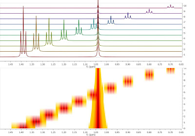
Crossing over of peaks is a very common event in Reaction Monitoring (RM) experiments. When this happens, the automatic alignment algorithm discussed in previous posts (here and here) might not work properly. To illustrate this issue, as I did not have a real experiment at hand, I simulated using Mnova a very simple data set comprised by a triplet and a singlet in such a way that the chemical shift of the triplet moves from 1.4 ppm to 0.7 ppm and having an exponential decay from spectrum to spectrum. This is depicted in the figure below, both as a stacked and a bitmap plot.

Now let’s say you are interested in extracting the intensities of the triplet as the reaction progresses. There is actually no need to pre-align the spectra algorithmically; it is much simpler to have some kind of graphical tool to instruct the software which peaks (or multiplets) need to be used for the reaction monitoring analysis. Let me show you how this works in Mnova:

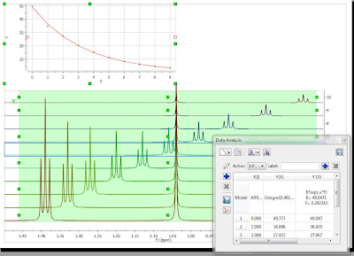
First of all, in the Data Analysis module you select the region to be analyzed. As a starting point, the region will have a rectangular shape (green rectangle in the figure below):

It can be noted that the graph shows an exponential decay, but the actual values must obviously be wrong as the values calculated, using the green rectangle as a boundary for the integration, include peaks from both the triplet and singlet, and we are interested in the analysis of the triplet resonances only. Now let’s change this…

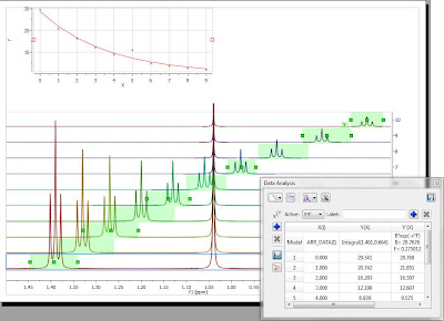
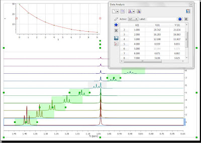
The selection rectangle has a number of handlers (small green boxes). You can drag and move them freely so that you can adjust the selection feature to follow the triplet (BTW, the number of handlers can be adjusted. In this case, there are 6 handlers, but higher numbers are also permitted). In the figure below, the result of adjusting the handlers to follow the triplet is shown:

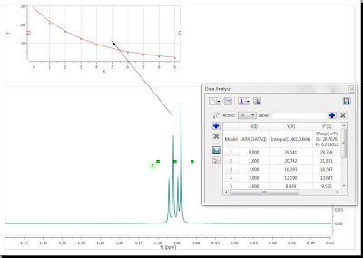
Now you can see that there is an outlier in the exponential curve which, obviously is caused by the singlet which overlaps with the triplet (spectrum number 6 which corresponds to data point #5, as in the graph the numbering starts from zero). Figure below shows that particular spectrum showing the singlet overlapping with the triplet:

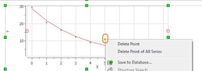
At this stage, there are several approaches. The simplest one is to just discard that point for the analysis, for example, by right clicking on that point in the graph and disabling it:

As soon as that point is deleted / disabled, Mnova will update the graph automatically. This is the new result:

Another approach would involve using GSD to eliminate the singlet from the triplet so that it would not be necessary to discard the information from that particular spectrum. However, this is something I will blog about in a future post.

Alignment of NMR spectra – Part V: Reaction Monitoring (I)

Previous posts on this series:
1. Alignment of NMR spectra – Part I: The problem
2. Alignment of NMR spectra – Part II: Binning / Bucketing
3. Alignment of NMR spectra – Part III: Global Alignment
4. Alignment of NMR spectra – Part IV: Advanced Alignment

Following the progression of chemical reactions by NMR is becoming more and more popular. Quoting Michael A. Bernstein et al. (Magn. Reson. Chem. 2007; 45: 564–571)

(…)The technique is rich in structural information, and can uniquely provide subtle information on speciation, protonation sites, and intermediate compound production. NMR measurements can be made under quantitative conditions, and one can be confident that all organic species will be observed. These factors combine to make NMR a very attractive tool for these analyses, and address many of the shortcomings in traditional spectroscopic measurements (…)

Typically, as a reaction proceeds, it’s very common to observe very significant chemical shift fluctuations of a given resonance due to, for example, changes in pH or protonation of the starting material, just to mention a few. These changes in chemical shift can be so large that extracting relevant information from those spectra (e.g. intensities/integrals across the data set) can be difficult, so aligning those spectra can be helpful. Let me illustrate this with an example exhibiting clear nonlinear misalignments: peaks at about ca 11.6 ppm do not move whilst the peaks at higher field move very significantly:



Instead of displaying the data set as a stacked plot as above, it might be more convenient to display it as an intensity or bitmap plot because this plotting mode highlights more clearly the alignment /misalignment profiles:



It’s evident that correcting the data using a single reference peak (or a global shift) is not sufficient. In order to align this data set, we can follow two different strategies:

Strategy 1:

Starting with raw spectrum (1), it is possible to perform a full-spectrum correction (global alignment) before the single intervals are aligned:



It can be appreciated that after applying the global alignment, most of the peaks in (2) are now properly aligned, except the peaks at the left which were previously aligned but after this operation get misaligned. This problem will be covered in the next step.
After the spectra have been aligned ‘globally’, the user just needs to select the interval which comprises the peaks left to be aligned as depicted in (1). (2) shows the final result once both the global and local alignment have been applied:



Strategy 2:

A different, although analogous strategy, would consist in aligning two different spectral intervals separately without resorting to a global alignment as shown in (1) below. Note that the peaks in the interval in the left are already well aligned (so selecting this region is optional; if there were some minor misalignment, the algorithm would optimize such residual misalignment).



(2) shows the final result after the two intervals have been aligned. It’s completely equivalent to the result obtained with Strategy 1

Conclusion
In this post I showed how the automatic alignment algorithm can be used to align RM data sets prior to any further analysis. However, there is a better way to extract NMR descriptors from Reaction Monitoring experiments that does not require any prior pre-processing alignment. In fact, I believe that this method, which I will present in my next post, has several advantages (in the context of reaction monitoring), especially in those cases where the chemical shift ordering of some peaks changes during the reaction, situations in which automatic alignment algorithms usually have great trouble dealing with. An example of a reaction monitoring data set showing peaks crossing over is shown below, in bitmap mode (it’s a simulated data set)


Therefore in my next post, I will show how to analyze RM data sets with important peak fluctuations and crossing over

Alignment of NMR spectra – Part IV: Advanced Alignment

Previous posts on this series:

1. Alignment of NMR spectra – Part I: The problem
2. Alignment of NMR spectra – Part II: Binning / Bucketing
3. Alignment of NMR spectra – Part III: Global Alignment

As I mentioned in my previous post, simple alignment based on shifting or referencing the whole spectrum is not enough in cases where there are different local chemical shift fluctuations.
Resorting back to the synthetic data set used in the previous posts, let me introduce a semi-automatic method designed specifically to align spectra having local chemical shift variations. From a practical point of view, the User needs to select the spectral regions to be aligned and then the program will automatically align those regions separately by using the same technique showed in my last post, that is, maximization of the cross-correlation function. The picture below shows the spectrum before alignment and the two selected regions (top) and the result obtained after applying the alignment algorithm (bottom).




Before going into the details of the automatic alignment algorithm, there is a point I think is worth mentioning: when you have several spectra to be aligned, it is necessary to specify the spectrum which will act as the reference (alignment target). Our implementation provides the capability to use as a reference any spectrum in the data set or the average spectrum.

Automatic Alignment: What is under the hood

Assuming that the spectral segments to be aligned are represented by two vectors g and h, a new vector f can then be generated by cross-correlation:


where * indicates the complex conjugate.
The cross-correlation implemented in Mnova is computed using the fast Fourier transform (FFT), which is a fast O(N log2[N]) process. Briefly, the strategy is to perform an FFT on each of the two vectors, invert the sign of the imaginary part of one Fourier domain representation of one of the vectors, multiply the two Fourier domain functions, and transform the result back using the inverse FFT. By simply calculating the index corresponding to the maximum of f(n) one can find the number of points in which vector g has to be shifted in order to get the highest cross-correlation with respect to h.
This is not, of course, the first time that cross-correlation has been applied for the alignment of two (or more) vectors. Actually, it has been extensively used for alignment purposes in many different contexts, including:

• Chromatography (Anal. Chem. 2005, 77, 5655-5661)
• NMR (J. Magn. Reson. 2010, 202, 190-202)
• DNA Sequence Alignment (J. Biomol. Tech. 2005, 16, 453–458)

The first article was the one that inspired me to include this method in Mnova and in fact, it was implemented several years ago as a method for the automatic alignment of 1D and 2D spectra (see this).
Very recently, we have improved the traditional cross-correlation algorithm by working on the first derivative domain calculated using an improved Savtizky-Golay routine in which the order of the smoothing polynomial is automatically calculated. The idea is to minimize potential problems caused by baseline distortions or very broad peaks.

We have found this method to be very useful not only in the context of metabonomics, but also in the alignment of Reaction Monitoring data sets. However, I better leave this topic for my next post …

Alignment of NMR spectra – Part III: Global Alignment

Previous posts on this series:

1. Alignment of NMR spectra – Part I: The problem
   
2. Alignment of NMR spectra – Part II: Binning / Bucketing
   

We have seen that binning helps in minimizing, for example, the effect of pH-induced fluctuations in chemical shift so that, in the field of NMR-based metabonomics studies, ensuring that signals for a given metabolite appear at the same location in all spectra. One evident disadvantage of binning is that it greatly reduces the spectral resolution (e.g. in a 500 MHz instrument, a typical 64 Kb NMR spectrum with SW = 12 ppm, would be reduced to 300 points (bins) if a bin width of 0.04 ppm [20 Hz = ~218 points] is used).
This loss of resolution is not desirable and considering that today’s powerful computers can handle large data matrices, there is now an increasing tendency to perform multivariate analysis at the maximum spectral resolution possible. Alternatives to binning typically involve some form of peak alignment procedure and in this post I will cover the simplest one, global alignment. The purpose of this post is to simply illustrate the concept of alignment, but it is important to note that this method is not generally applicable to the misalignment problems found in metabonomics NMR data sets, although it might be useful in many other contexts.

The idea of global alignment is very simple and corresponds to the well-known chemical shift referencing method in which the user sets the internal reference peak (e.g. TMS, DSS, TSP, etc) of each spectrum to e.g. 0 ppm. In order to cope with small fluctuations in chemical shifts, this method seeks for the highest peak within a narrow (user-defined, auto-tuning option in Mnova) interval, as depicted in the figure below:



Clearly, this method will not work properly in those data sets with local misalignments, that is, when signals of one metabolite fluctuates in one direction whilst the peaks of a different metabolite move differently). As an example, let’s consider again the simulated data set of Taurine used in my previous post and which I copy below for convenience:



Remember that this data set has been generated by randomly changing the chemical shifts of the two CH2 groups. Now, let’s apply the global alignment procedure using as chemical shift reference at a value of 3.25 ppm as shown in the picture below:



As expected, all peaks corresponding to the triplet at 3.25 get perfectly aligned, but the other multiplet remains misaligned (see below).



One could devise an extension to this global alignment procedure in which the same procedure is applied to different segments of the spectrum. In this particular case, one could select two different windows, one for each triplet and apply the same algorithm locally to each segment. However, having to manually select the chemical shift reference for each segment is not very practical and, in addition, relying only on the simple search of the maximum peak within each segment is not a very robust method for automatic alignment. In my next post, I will present a much more powerful automatic alignment method in which the user will not need to define the reference chemical shift value for each segment / window, but before that, and as an introduction to that post, let me show you another global automatic alignment method.
Let’s assume that we have several spectra which we want to align automatically in such a way that we first manually reference the chemical shift of one of these spectra (e.g. the first one in the series) and then ask the software (e.g. Mnova) to automatically align all the other spectra using this one as a reference spectrum. The idea for such algorithm is to figure out which is the optimal value that a spectrum has to be shifted (left or right) so that the difference between this spectrum and the reference one is minimal.



Such alternative ‘global method’ has been implemented in Mnova several years ago already and is based on the maximization of the cross-correlation between the reference spectrum and the spectrum/spectra to be aligned. This procedure is the essential foundation for the advanced alignment method which I will present in my next post.

Alignment of NMR spectra – Part II: Binning / Bucketing

In my last post, I wrote that spectra of biological samples are usually poorly aligned due to wide changes in chemical shift arising from small variations in pH or other sample conditions such as ionic strength or temperature.

The most widely used method of addressing this chemical shift variability across spectra is by means of the so-called binning (or bucketing), procedure that consists in segmenting a spectrum into small areas (bins / buckets) and taking the area under the spectrum for each segment. Preferably, the size of the bins should be large enough so that a given peak remains in its bin despite small spectral shifts across the spectra, but not so large as to include peaks belonging to multiple compounds within a single bin.
As a simple example to illustrate how binning works, let’s consider the spectrum of Taurine (Fig. 1)

Fig. 1: 1H-NMR spectrum of Taurine synthesized with Mnova NMRPredict. Only the spectral region corresponding to the methylene protons is shown.

Taking the spectrum shown in Fig. 1 which has been predicted using Mnova NMRPredict, seven additional spectra were created by changing the chemical shift of the CH2 protons randomly in an effort to simulate the chemical shift variability observed in real life biofluid NMR spectra.

Fig. 2: Synthesized data set comprised by 8 simulated spectra of Taurine with random chemical shifts for the CH2 protons and displayed in superimposed mode in Mnova.

These spectra have been synthesized using 32768 data points and a spectral width of 6001.6 Hz with a spectrometer frequency of 500.13 MHz. If the size of each bin is set to 0.02 ppm (represented by the vertical grid lines in Fig. 2), this will result in the generation of 6001.6 / (0.02 x 500.13) = 600 bins.

When the binning command is issued in Mnova, a new spectrum with 600 data points in which every point is the sum of all the points within each bin is produced. The result of this binning or bucketing operation applied to one single spectrum of the synthetic Taurine data set is depicted in fig. 3, where the circles correspond to the area of each bucket in the original spectrum. Fig. 4 shows the result applied to all spectra in superimposed mode. Digital resolution of the resulting binned spectrum is 10 Hz/point

Fig. 3: Methylene region of one synthetic 1H-NMR spectrum of Taurine after data reduction by uniform binning

Fig. 4: Result of applying data reduction by uniform binning to the 8 1H-NMR spectra of Taurine

Once the spectra have been binned, they are ready to be exported in a convenient format (e.g. ASCII) for further statistical analysis (e.g. PCA).
It can be noticed that binning greatly minimizes the effects from variations in peak positions (in this case, all peaks get perfectly aligned). Additionally, binning reduces the data size for multivariate statistical analyses, although today’s computers and optimized linear algebra algorithms are able to handle large data volumes very efficiently.

The major drawback of this procedure is the loss of a considerable amount of information enclosed in the original spectra. In this particular case, the fine structure of the two triplets is totally lost (the coupling constant is 6.6 Hz whilst the digital resolution is 10 Hz), precluding the direct interpretation of multivariate models. In addition, peaks moving on borders between bins might cause artifacts. Another source of loss of information occurs, for example,when peaks belonging to several compouns are included within a single bin.

There exist several better alternatives to binning, typically involving some form of peak alignment without data reduction. But this will be the subject of my next post …

Alignment of NMR spectra – The problem: Part I

The chemical shift is of great importance for NMR spectroscopy because it reflects the chemical environment of the nuclides under observation providing detailed information about the structure of a molecule.

Although the chemical shift of a nucleus in a molecule is generally assumed to be fairly stable, there are a number of experimental factors (pH, ionic strength, solvent, field inhomogeneity –bad shimming, temperature, etc) which might produce slight or even quite significant variations in chemical shifts.
This is particularly important in metabonomics/metabolomics where shifts of NMR peaks due to differences in pH and other physico-chemical interactions are quite common in NMR spectra of biological samples. For example, some important metabolites, such as citrate or taurine, have peaks whose chemical shifts fluctuate in an uncontrolled way from sample to sample. These variations can cause spurious grouping of samples in chemometric models.

Example of peak position variation in the citrate region (simulated data)

Whilst it is critical to setup the experimental conditions in the best way to minimize these chemical shift fluctuations (for example by using an appropriate buffer; BTW, there exists a standard protocol for biofluid [urine, serum/plasma] and tissue sample collection and preparation as described by Beckonert et al. [1]), spectral misalignments may still occur and special post-processing methods have to be employed.
Another example in which variation in the chemical shift is important occurs in the context of kinetics or reaction monitoring experiments by NMR. For example, consider the following reaction monitoring example [2]:

Reaction monitoring data set for the solution of phenylethylamine and 2-methoxyphenyl acetate in D2O, with every 35th spectrum from the first (bottom) to the last (top) shown (see [2])

It can be appreciated that during the course of the reaction, the chemical shifts of several signals change as a result of the change in pH (in this case, as a hydrolysis proceeds)
Although characterizing these chemical shifts fluctuations can be sometimes important (pH or drug binding-induced chemical shifts, for example) in general they obscure the process of pattern recognition (metabonomics) and impede the performance of data analysis (e.g. selection of the peaks whose intensities/heights need to be monitored becomes more difficult).

In my next posts, I will cover different ways to deal with the peak misalignment problem, first in the field of metabonomics and then in reaction monitoring.

References:
[1] O. Beckonert, H.C. Keun, T.M. Ebbels, J. Bundy, E. Holmes, J.C. Lindon, J.K. Nicholson, Metabolic profiling, metabolomic and metabonomic procedures for NMR spectroscopy of urine, plasma, serum and tissue extracts, Nat. Protoc. 2 (2007) 2692–2703

[2] M. Khajeh, M. A. Bernsteinb, G. A. Morrisa, Magn. Reson. Chem. 2010, 48, 516–522

Here I am again!

As you've undoubtedly noticed there has been little activity on my blog lately, which contrasts with the high activity I'm having in my real life, with a plethora of exciting (and challenging) new projects going on in my company, Mestrelab Research.

One particular area in which we have been working on quite intensively for the last few months belongs to the broad subject of the alignment of NMR spectra. This appears to be a very important topic for those scientists working, amongst others, on fields like metabonomics/metabolomics and reaction monitoring by NMR. Starting from today, I will start blogging about this issue, firstly covering some very basic concepts and then moving on to some more advanced techniques for the efficient alignment of NMR spectra.

So stay tuned!