Binning and NMR Data Analysis

Yesterday I mentioned that many NMR arrayed experiments suffer from unwanted chemical shift variations due to fluctuations in experimental conditions such as sample temperature, pH, ionic strength, etc. This phenomenon is very common in NMR spectra of e.g. biofluids (metabonomics/metabolomics) but also exists in many other experiments such us Relaxation, Kinetics and PFG NMR spectra (diffusion).

This problem negatively affects the reliability of quantitation using, for instance, peak heights, and for this reason integration is, in general, a more robust procedure as these spectral variations are mitigated by averaging data points over the integral segment. In this post, I just want to show you one simple trick which helps to understand, in a pictorial way, why integration is useful to remove the major part of chemical shift scattering.

First, consider the following experiment depicted in the figure below. It shows a triplet and as you can see, some minor peaks shifts are present from spectrum to spectrum

If peak heights are determined at a fixed position, this might introduce appreciable errors in the posteriori quantitative analysis (e.g. exponential fitting). As described in my former post, this could be circumvented in some extent by using parabolic interpolation or peak searching of the maximum in a predefined box.
Nevertheless, integration is a very simple solution as can be appreciated in the figure below. Instead of using the Peak Integrals tool in the Data Analysis module, I will show now a complementary procedure. Basically, what I have applied to all spectra is the well-known binning operation which consists of dividing each spectrum in equally sized (e.g. 0.01 ppm in this case) bins, so that integral (area) of each bin represents a new point in the binned spectrum


As seen in the figure above, binning clearly removes the effect of chemical shift changes but of course, at the cost of a significant reduction in data resolution.

Basics on Arrayed-NMR Data Analysis (Part IV)

Next up in my survey on analysis of arrayed NMR experiments ( View Parts 1, 2, 3 ) takes me to a quick overview of the different methods of data evaluation, such as the determination of peak heights and peak areas from arrayed experiments. Here you go...

---

Of the different existing methods for the extraction of peak intensities from arrayed NMR spectra (see [1] ), Mnova provides the following ones:

(1) Peak area integration

This is the default method in Mnova Data Analysis module (see figure below)


This method consists of a standard numeric integration over the whole peak. Basically, the program is summing up all the points within the selected area of interest) as illustrated in the figure below:

This figure has been created as follow: two identical Lorentzian lines (green & red) were simulated and then noise was added. The noise level is the same in both spectra but obviously, the actual numbers are different (more technically, noise in both spectra was calculated using a different seed in the random number generator).

This peak area method for data extraction is quite robust to noise (provided that the noise level is more or less constant across the different spectra in the arrayed experiment) and more importantly, insensitive to chemical shift fluctuations from trace to trace in the experiment, a situation which is more frequent than generally realized. For these reasons, and for its simplicity of use, this is method of choice for well-resolved peaks.

If the peaks of interest exhibit some degree of overlap, this method is not very reliable and some of the next methods will be more convenient

(2) Peak Height Measurement

This is the second method for data extraction (see figure below) and it finds the peak height at a given chemical shift across all the spectra in the arrayed experiment.


By default, the program will find the peak intensity at the position indicated by the user (using a vertical cursor) and then it will perform a parabolic interpolation in order to refine the value. In addition, the user can specify an interval in such a way that the program will find the maximum peak within that region. This can be done in 2 different ways:

• i) If you click in the Options button, you can define whether you want to use Parabolic and the interval in which the maximum should be found (in ppm

• (ii) Alternatively, once a peak has been selected, you can change the interval by direct editing of the peak selection model. In the figure below, I’m showing how the peak selection model is PeakIntensity. The first number (6.001 in the figure) corresponds to the central chemical shift whereas the second number (0.100 in the figure) represents the interval for the peak maximum search.

Parabolic interpolation is useful because it minimizes the problems caused by the random noise. For example, let’s assume that Parabolic interpolation is not used so that peak heights extraction will be done always at the same fixed chemical shift position (see figure below). As described in reference [1] and illustrated in the figure below, when this method is used the values are seen to be quite different in the two cases: here the precision of the measurement will depend strongly on the noise.

Parabolic interpolation and/or measurement of the intensity as the maximum height within a fixed box around the peak will help to minimize the effects of movements on the chemical shift position of the peaks due to, for example, temperature instability, pH changes, etc.

For convenience, Mnova includes the so-called Pick Max. Peak method which is totally equivalent to the previous one but it allows the graphical selection of the left and right boundaries in which the maximum peak will be searched for.

In a nutshell, peak height measurement can be used in those cases in which peak overlap might represent a problem. However, it should be noted that if for some reasons the line widths of the peaks under analysis change from trace to trace, peak heights will not represent a reliable measurement and peak integrals should be used instead.

In general, I would recommend peak integrals as the most general-purpose method for quantitation of peak intensities in arrayed experiments.

In the next post of these series I will address the problem of exponential fitting useful in relaxation and diffusion experiments.

References:

[1] Viles JH, Duggan BM, Zaborowski E, Schwarzinger S, Huntley JJA, Kroon GJA, Dyson HJ, Wright PE. 2001. Potential bias in NMR relaxation data introduced by peak intensity analysis and curve fitting methods. J Biomol NMR 21:1–9 (link)

Basics on Arrayed-NMR Data Analysis (Part III): Extracting and calculating useful NMR related molecular information

After the basic introductory posts on arrayed NMR experiments, it’s now time to get some action and see how to extract relevant information from these experiments and calculate useful NMR related parameters such as diffusion, relaxation times, kinetics constants, etc.

Actually, in this post I will cover the first case, that is, the analysis of PFG experiments to calculate diffusion coefficients. The reason for this is twofold: (1) I have a nice PFG data set whilst the quality of the relaxation experiments I currently have access to is quite poor (if any of you have any good relaxation data and can send them over, I would be very grateful) (2) The current version of Mnova has been optimized to handle PFG experiments fully automatically whilst some simple manual intervention is needed when working with other arrayed-like NMR experiments. However, I would like to emphasize that, for example, relaxation experiments are already fully supported in the current version of Mnova, although it is necessary to enter the time delays manually in the program (this is very simple, btw). Automation of relaxation experiments is already possible with alpha versions of Mnova.

This is how a PFG experiment can be analyzed with Mnova with the Data Analysis module (for your information, Mnova includes a DOSY-like processing algorithm based on a Bayesian Algorithm. See this http://mestrelab.com/dosy.html and this http://nmr-analysis.blogspot.com/2008/09/baydosy-whats-under-hood.html for more information):

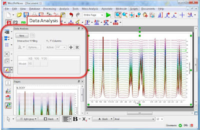
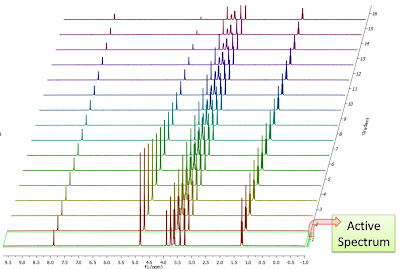
Once the arrayed spectra has been loaded into Mnova, issue menu command Analysis/Data Analysis. The so-called Data Analysis widget will popup. This will be the central control panel (see figure below) for anything related to the analysis of arrayed experiments.

Its operation is very simple. The first thing you have to do is click on the New button. As a result, Mnova will populate the X-Y Table with some initial values (as described in a moment) and create a new item, the so-called Data Analysis Plot. This new item will display the values from the X-Y Table which in general are the values extracted from the arrayed spectra, both experimental (Y) and fitted (Y’).

The X-Y Table

This table is composed by one X column, X(I), one or several Y-columns (Y, Y1, Y2, etc) to hold the experimental values extracted from the arrayed spectra and one or several Y’-columns which hold the fitted values of their Y counterpart columns.

X-Column

When the table is initialized, in the case of PFG experiments the X-column is populated with the Z values from the Diffusion table, that is, the gradient strengths scaled by taking into account the constants from the selected Tanner-Stejskal model. In the case of a relaxation experiment, the X column will contain the time delays. Of course, it is possible to change the contents of the X-column by following any of these methods:

• Manual editing of the individual cells

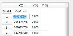
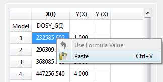
• Copy & paste from a text file. For example, you can put the values for the X-column into a text (ASCII) file and then paste its contents into the table. To do that, just right click on the first cell you want the paste action to start from.

• Enter a formula into the Model cell. Double click on the X(I) model cell (1) and then enter the appropriate equation to populate the X column (2). For example, if you simply enter I, the X column will be filled in with numbers 1, 2,3, etc. If you enter a formula like 10+25*I, the X column will be filled with numbers 35,60, 85, etc.

Y-Column

In all cases, when the table is initialized, the Y-column is automatically filled in with values 1,2,3, etc. The purpose of this column is to hold the experimental values from the arrayed experiment. For example, in the case of a PFG experiment, it may contain how the intensity (or integral) of a given peak (or set of peaks) evolves as the applied pulse field gradient changes. Likewise, in the case of T1/T2 experiments, this column will show the relaxation profile of a given resonance (or set of resonances). So the question is: how to populate the Y-column with actual information from the spectra?

This is again very easy. There is a graphical way (mouse driven) and a manual one. Let’s start with the graphical method:

• Graphical Selection: Click on the ‘Interactive Y Filling’ button (see red-highlighted button in the image below). After doing this, the cursor will change into an integral shaped cursor expecting you to select the region from where you want the integrals to be extracted across all the subspectra in the arrayed item. After the selection is done (see figure below), all the integrals will be placed in the Y column and those values will be displayed in the X-Y plot as green crosses (note: the shape, color, etc of these crosses can be customized from the X-Y plot properties).

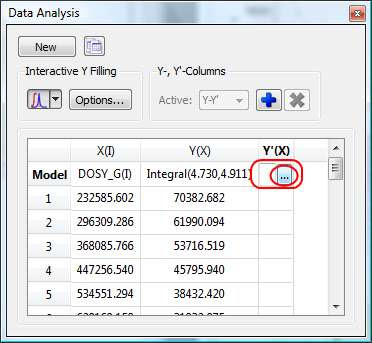
• Manual selection: if you take a closer look at the Data Analysis table in the figure above, you can appreciate that once the integral region has been selected, the program shows the following text: Integral(4.752, 4.907). This means that we have selected an integral covering that range. This value can be edited manually so that you can specify the limits by simply editing that cell.

Y’-Column

The Y’ column is reserved for the fitted values assuming a particular theoretical model (e.g. a exponential decay). In this particular case, as we are dealing with PFG experiments, we will be interested in the calculation of the Diffusion coefficients and thus, our fitting model could be a mono-exponential decay (multi-exponential decays can also be handled with this module, but I will not address this problem in this post). The process is very simple:

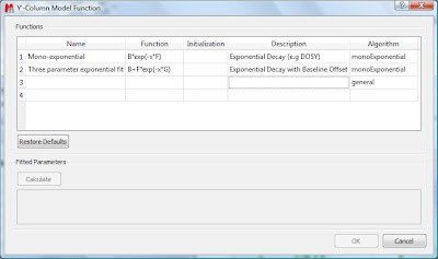
First click on the Y’(X) cell and then on the small button with 3 points as indicated in the figure below.

This will launch a dialog box with powerful fitting capabilities.

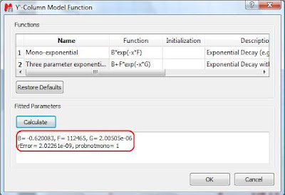
This dialog provides two predefined functions useful for fitting mono-exponential data (such as PFG and Relaxation NMR experiments) using either a 2- or a 3-parameter fit. Furthermore, this dialog offers the possibility to enter user customized functions. As this post is already taking too much space, I will leave the details on data fitting for the next post. For the time being, suffice to say that if your problem regards mono-exponential functions, just select any of the 2 predefined functions in the dialog box and click on the Calculate button. Mnova will immediately compute the optimal values, returning these optimal values as well as the fitting error) and the probability that the acquired series follows the chosen monoexponential model.

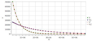
Finally, after closing the dialog, it will populate the Y’ column and the X-Y will be updated with the fitted curve (Red line in the figure below).

One nice feature of the Data Analysis module is its ability to handle multiple series. For example, it’s possible to analyze the decay of several resonances within the same experiment. In order to do that, just click on the (+) button to add a new series and repeat the same process to select the desired resonance range and fit the values. For example, in the figure below I’m showing two curves with different decay rates.

In my next post I will cover some more details about the different methods available to select the intensities/integrals from the spectra and some basic points on the fitting algorithm.
BTW, you can download the full PFG data set used in this post

Basics on Arrayed-NMR Data Analysis (Part II): Practical hints

Further to my previous post, I will cover today some more basic tools available in Mnova for the analysis of NMR arrayed experiments. In particular, I will touch on the following points:

• How to use different display modes for 1D arrayed spectra
• How to navigate throughout the different subspectra in the arrayed item
• How to process individual spectra separately

When an arrayed experiment has been detected, all subspectra are grouped together and plotted in the stacked display mode in Mnova (see figure below). Several points are worth mentioning:

(A). Take a look at the green box in the figure below: it shows the so-called ‘active spectrum’. What does this mean?

The concept of active spectrum is easier to illustrate with the following example: as I wrote in my previous post, in general all the spectra in an arrayed item are processed exactly with the same processing operations. For example, same level of zero filling, same apodization function, same FT type, same phase correction, etc. However, it i’s possible that some particular spectra require a slightly different processing, independently from the others. In order to do that, it i’s necessary to deactivate the ‘Apply Processing to All spectra in Stack’ option.

So if that option is off, any processing operation will be applied only to the active spectrum in the stack.

The question is: how can we change the active spectrum? There are 3 different ways:

1. Just click on the spectrum you want to be active. This is probably the most intuitive way.
2. Use SHIFT + Mouse Wheel to navigate throughout all the spectra in the stack, one after the other.
3. Use SHIFT + Up/Down arrow keys. This is analogous to point 2)

(B). If the number of subspectra (traces) is large (e.g. > 10), working in the stack mode might not be very practical. Quite often, working only with the active spectrum on the screen will be a much better option. This mode can be activated as shown in the image below.

While working on this mode, you will see on the screen just the active spectrum. Should you want to move to another spectrum without resorting to the stack mode, just use methods 2) and 3) described above (Shift+Mouse Wheel or Shift + Up/Down keys).

IMPORTANT: Remember that even if only the active spectrum is visible, unless the “Apply Processing to All spectra in Stack” option is off, all spectra in the stack will also be processed.

(C) Another useful display mode consists of superimposing all subspectra (see figure below). This method is very useful, for example, when you want to check whether some peaks shift their position (for instance, due to differences in pH, temperature, etc., as is common in biofluids spectra).

Finally, there is an additional display mode, the so called whitewashed stacked plot. The whitewashing effect means that the spectra at the front of the display hide the spectra behind them from view, as depicted in the figure below.

This plotting mode can be useful to create nice reports, but it’s important to emphasize that drawing time will be significantly higher than with the other plotting modes, so it is not recommended when processing the spectra in real time (e.g. interactive phase correction).

In my next post I will show how to extract useful information from arrayed spectra.

Basics on Arrayed-NMR Data Analysis (part I)

In this post I will cover some basic concepts on the analysis of a very important class of NMR experiments, the so-called Arrayed NMR spectra. The concept is very simple: an arrayed experiment is basically a set of individual spectra acquired sequentially and related to each other through the variation of one or more parameters and finally grouped together to constitute a composite experiment. These experiments are also known as ‘pseudo-2D’. For example, in the case of Bruker spectra they have the same file name as 2D spectra, that is ser files (ser = serial spectra) . In the case of Varian, the file name is fid (Varian uses the same name for 1D, 2D, 3D, … and arrayed spectra). However, unlike with actual 2D spectra, arrayed spectra are only transformed along the F2 –horizontal or direct- dimension (assuming 1D arrayed spectra only).

The modus operandi is better explained with an example: let’s suppose it is necessary to acquire a pulse field gradient (PFG) experiment. Instead of acquiring independent spectra, it is more convenient to create an array with increasing PFG amplitudes. All resulting spectra are now treated as a single experiment. This grouping greatly facilitates processing as, in general, all subspectra require the same processing operations (apart from some occasional minor adjustments of one or several spectra). More about this in a moment.

Well known examples of NMR arrayed experiments are, among others:

• Relaxation (T1, T2)
• PFG experiments (DOSY)
• Kinetics and reaction monitoring by NMR

Any good NMR processing software should be able to automatically recognize when an NMR spectrum is an arrayed experiment and will setup all processing operations accordingly. For example, the figure below illustrates the results obtained when a Bruker arrayed folder is dragged and dropped into Mnova:

What has happened here are basically 2 things:

1. First, Mnova detects that the dropped folder contains an arrayed experiment
2. With that knowledge in hand, Mnova proceeds to process all the individual spectra, one after the other and of course, along the only valid dimension (F2). So for every spectrum, Mnova applies appropriate weighting, zero filling, FT, phase correction, etc and stacks all the spectra as shown in the picture above

As a result, all individual spectra grouped within one composite item (i.e. arrayed item) have been processed in the same way. However, it’s very common that some subspectra might require independent tuning. For example, many PFG NMR experiments present gradient dependent phase shift so that it becomes necessary to adjust the phase of some individual spectra separately. This is very easy to accomplish with Mnova and it will be the subject of my next post.