Chemometrics under Mnova 9 - PCA

(Note: This entry has been written by Dr. Silvia Mari, from R4R who has helped us to design and implement this module)

Background: spectroscopy and chemometrics

“For many years, there was the prevailing view that if one needed fancy data analyses, then the experiment was not planned correctly, but now it is recognized that most systems are multivariate in nature and univariate approaches are unlikely to result in optimum solutions.”

      Hopke, P. K. (2003). The evolution of chemometrics. Analytica Chimica Acta, 500(1-2), 365–377]
  
Either we apply analytical chemistry for quality and control or we attempt to a more “system biology” approach for our R&D we do need advanced methods to design experiments, calibrate instruments, and analyze the resulting data. And the “emergence of chemometrics thinking came from the realization that traditional univariate statistics is not sufficient to describe and model chemical experiments”
       Geladi, P. (2003). Chemometrics in spectroscopy . Part 1 . Classical chemometrics, 58, 767–782

With this in mind Mnova 9 now offers to its users a module called PCA which could be found under the main menu “Advanced”. It is the result of our first efforts to include chemometric tools into Mnova and it is meant to give spectroscopist the possibility to interactively work on both stacked spectra and its corresponding statistical plots.

Starting from mid ‘70s where the first paper with chemometrics in the title appeared in 1975 [1], chemometrics has grown up and is now considered a functioning research area in the chemical science. It has expanded widely from its beginnings into a variety of other areas including multivariate calibration, pattern recognition, and mixture resolution and today there are several applications of interest for the NMR spectroscopists [2-5].

PCA module

Principal Component Analysis (PCA) is a procedure which uses orthogonal transformation to convert a set of observations from correlated variables into a set of values of linearly uncorrelated variables (named principal components) [6].

PCA module under Advanced menu is working in two subsequent steps: (1) matrix generation and (2) principal component analysis. The overall workflow can be represented with the following illustration, where general steps available in Mnova are highlighted in blue whilst specific functionalities of this new PCA module are highlighted in yellow.

With the aim to help the spectroscopist to refine and optimize the data matrix to be used for advanced analysis, PCA in Mnova makes it very easy the detection and removal of spectrum outliers, reveal problems in spectral alignment as well as in its phase or baseline. Once the user has properly corrected those regions of interest, the PCA module allows to re-run the analysis, either replacing the previous analysis or creating a new one for comparison.

Interaction with the stacked spectra.

The main effort applied during the design and development could be summarized in one word: SYNCHRONIZATION. PCA plots, PCA tables and stacked plot are always synchronized. By doing so selections of a point in the score plot imply a selection in the stacked plot. 

In the same way, a selection of a point in the loading plots (hence a selection of a variable of the matrix) generate a shadow into the stacked plot according to the bin position and size.

Colors and graphics

When dealing with large dataset, color coding plays a very important role and eventually essential. Even if PCA does not use class definition in its algorithm since it is an unsupervised method, the kind of patterns expected is generally known.

The driving concept here is that colors are assigned on the basis of class belonging. Again, as in the previous section, colors are always synchronized from PCA tables to PCA plots and to stacked spectra as well

Moreover, in the loading plot, the user is allowed to select more than one bin (see flag option in the loading plot table, or multiple selection of table entry using shift or ctrl  key). Visualization of a bin region is obtained with a colored box that is displayed superimposed over the stacked plot. The User can associate different colors to different bins regions

Data filtering and scaling

The results of the analysis depend on the types of filtering and scaling of the matrix that user selects, which therefore must be specified. It can be demonstrated how both factors greatly affect the outcome of the data analysis and thus the rank of the most important variables. PCA module includes several possibilities in terms of data cleaning and scaling.

There is not a general rule in the selection of the type of scaling. For that purposes we recommend the manuscript from van den Berg et. al. [7] which describes extensively how these transformations could improve the information content of the data matrix. Finally, bear in mind that visual inspection and assessment is ultimately one of the most important steps in chemometrics.

Conclusion

We have introduced in Mnova 9 a chemometric module called PCA (Principal Component Analysis). PCA have been shown to be very effective in compressing large volume of noisy correlated data into a subspace of much lower dimension than the original data set. Data pretreatment method is crucial to the outcome of the data analysis. The resulting low dimensional representation of the data set has been shown to be of great utility for analysis or monitoring the system under study, as well as in selecting variables for control or markers of the expected pattern.

The possibility to interactively play with PCA plots and spectra at the same time, and the user friendly interface provided by Mnova will be of great advantages also for spectroscopists that are not familiar with multivariate analysis but would like to learn more and test it.
As has always been for Mnova community, the future of this new first step in chemometrics will be driven by user requirements. For that reason we look forward to get feedback, criticisms, suggestions, comments and lots of requests for future development. So, play with it and have fun at looking at your own datasets from a different perspective!

References

[1] B.R. Kowalski, Chemometrics: views and propositions, J. Chem. Inf. Comp. Sci. 15 (1975) 201–203

[2] Chemometrics in bioreactor monitoring. Lourenço, N. D., Lopes, J. a, Almeida, C. F., Sarraguça, M. C., & Pinheiro, H. M. (2012). Bioreactor monitoring with spectroscopy and chemometrics: a review. Analytical and bioanalytical chemistry, 404(4), 1211–37. doi:10.1007/s00216-012-6073-9

[3] Metabonomics and chemometrics in food science and nutrition. Kuang, H., Li, Z., Peng, C., Liu, L., Xu, L., Zhu, Y., Wang, L., et al. (2012). Metabonomics approaches and the potential application in food safety evaluation. Critical reviews in food science and nutrition, 52(9), 761–74. doi:10.1080/10408398.2010.508345

[4] Pharmaco-metabonomic phenotyping and chemometrics. Robertson, D. G., Reily, M. D., & Baker, J. D. (2007). Metabonomics in Pharmaceutical Discovery and Development, 526–539.

[5] Metabonomics and chemometrics in drug safety and toxicology. Griffin, J. (2004). The potential of metabonomics in drug safety and toxicology. Drug Discovery Today Technologies, 1(3), 285–293. doi:10.1016/j.ddtec.2004.10.011

[6] Principal component analysis, Svante Wold, Kim Esbensen, Paul Geladi. Volume 2, Issues 1–3, August 1987, Pages 37–52

[7] Van den Berg, R. A., Hoefsloot, H. C. J., Westerhuis, J. A., Smilde, A. K., & van der Werf, M. J. (2006). Centering, scaling, and transformations: improving the biological information content of metabolomics data. BMC genomics, 7(1), 142. doi:10.1186/1471-2164-7-142

Chemical Shift, Absolutely!

(Note: This entry has been written by Dr. Mike Bernstein - Thank you, Mike!)

It’s a “given” that for NMR the chemical shift must be reported relative to standard. The most widely used is the 1H signal of tetramethylsilane (TMS) in chloroform, which has an assigned value of exactly zero. This is convention, and we all adhere to it. Correctly referencing 1H NMR spectra is seldom a difficulty, whether we use co-dissolved TMS (or a water-soluble equivalent), or the residual proton signal from the deuterated solvent. Things can get more complex, but this works for the vast majority of us. The chemical shift, d, is defined thus:

Venturing to the “dark side” of NMR – nuclei other than 1H – seldom stretches beyond 13C for most, and a residual solvent signal is very often present that can be used as a secondary chemical shift reference. But beautiful possibilities tempt many of us. Whether you are interested in biomolecular NMR and live and breathe 15N and possibly 31P, or 2H, or an orgametallic chemist with an interest in far more exotic nuclei, each heteronucleus has its charms and challenges. One thing unites NMR of all nuclei: adherence to a convention for chemical shifts. This can be easier said than done, given that some reference materials are difficult to handle, expensive, etc. The chemical shift reference compound for 19F NMR is the banned substance, Freon-11.

Absolute chemical shifts

We get help from a group working under the IUPAC [1] guise for their work in helping us calculate the chemical shift scale for all NMR-active nuclei [2].  That is, they provide us with a standard way to get the chemical shift precisely correct for any and all heteronuclear NMR spectra. That’s amazing - and hugely useful!

So how does it work? Well, it’s quite simple, really. At the heart of the calculation is the absolute frequency of the 1H signal of TMS for your NMR spectrometer hardware (console, probe, etc.) and sample (solvent, temperature, etc.). You need to be able to determine the exact frequency of this reference signal to seven decimal figures, at least. The following equation applies (sometimes expressed as a percentage) and uses a ratio to describe a constant, X (Greek capital Xi):

Making it easy with Mnova

We make heavy use of absolute referencing (AR) in Mnova, with the following available:

• Correctly reference an X-nucleus spectrum when the referenced 1H spectrum is available
• Apply AR to heteronuclear axes in 2D experiments
• Allow users to customise the X  values
• Indirect 1H spectrum referencing using n_TMS  for a specific hardware and solvent (locked)

Referencing heteronuclear spectra

Ensure that you have a document having (a) a correctly referenced 1H NMR spectrum, and (b) one or more –nucleus spectra.

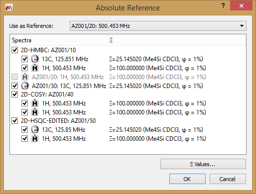
Select Analysis è Reference è Absolute reference… and choose the X-axis spectrum/spectra to reference.  

The table of X values

Note that by tapping on the “X values…” button you will be presented with the table of X-nuclei. In the case of 15N, for example, you can choose which reference standard you want to use. By clicking on the blue “+” button you can enter your own, customised value. 

Referencing 2D spectra

When there are 2D spectra in the document then the Absolute reference… selection will reflect this, and allow you to choose which spectrum is used for referencing purposes, and the traces to which this should be applied. Note that you can adjust the referencing of 1H and X-nuclei.

Referencing a 1H spectrum

You can use saved n_TMS values to reference another 1H spectrum from the same NMR spectrometer. Start with a correctly-referenced 1H NMR spectrum, and select Analysis è Reference è Edit saved references…  From this dialogue you can add the value for the particular hardware and measurement conditions – solvent, temperature, etc. 

Now, when you select Analysis è Reference è Apply saved reference then the saved value will be used if the criteria are met. 

Conclusions

Absolute referencing is a powerful way to ensure that data are correctly referenced. This is equally important in open-access environments as it is under automation, where it helps processes such as Verify be more robust. 

References

[1] (a) Harris RK, Becker ED, Cabral de Menzes SM, Goodfellow R, Granger P. Pure Appl. Chem. 2001; 73: 1795

(b) Harris RK, Becker ED. J. Magn. Reson. 2003; 156: 323.

[2] This is nicely described here: http://www.chem.wisc.edu/~cic/nmr/Guides/Other/Xi_chem_shift_scale.pdf

Copy and Paste NMR spectra

This is just a short entry to illustrate one nice little tool in Mnova NMR that I believe can be very handy in many situations.

Let’s suppose you have an NMR spectrum in which you have spent some time trying to customize its visual aspect. For example, you have changed the default line color and width, hidden the vertical scale, modified the background color, customized the chemical shift scale, etc. As a result, you may have something like this:

   

Now you open a new spectrum and you find that it is using the old default graphical properties and you want that this spectrum has exactly the same visual aspect as the previous one. 

There are several ways in Mnova to achieve that goal. For example, you can go to the first spectrum, go to spectral properties and save these properties to a file which can then be loaded in the target spectrum. 

However, in this post I want to show a simple shortcut that yields the same result. The procedure is as simple as this:

  

1) Go to the first spectrum and press Ctrl+C (Edit / Copy)

2) Move to the second spectrum and issue this command: Edit / Paste Properties / NMR Graphic Properties 

This is it, the second spectrum will have now the same visual aspect as the first one. 

The same trick can be used to copy and paste integral regions, zoom & cuts regions, etc.

Reference Deconvolution

Introduction

In an idealized situation, according to quantum mechanics theory, NMR transitions in liquid state and excluding dynamic effects such as chemical exchange are of Lorentzian shape [1]. In practice NMR lineshapes are never pure Lorentzians due to a number of reasons [2], ranging from magnetic field inhomogeneity and magnetic field noise to sample temperature gradients, sample spinning  or FID weighting, to cite a few. 

Another important property that might affect significantly the final observed lineshape is the following: Even in molecules of modest size the number of distinct peaks might be thousands times smaller than that of quantum transitions. As a simple example, the number of transitions of a molecule containing 15 would be 245760 whereas only a few hundreds of peaks would be observed in the spectrum. As a result, an NMR peak is actually an envelope of a distribution of myriads of Lorentzians and its shape is dominated by the coupling pattern of the spin system. 

Whilst this kind of line broadening affects signals differently across the spectrum and is very difficult (or even impossible) to resolve by post-processing operations, there are many other distortions that affect all resonances in the spectrum in the same way. These include lineshape distortions caused by poorly shimmed samples and they can be removed by using a post-processing technique known as Reference Deconvolution [3] 

Reference Deconvolution

This technique is used to remove the instrumental lineshape distortion by deconvolving the experimental NMR spectrum using a reference signal, usually one within the same spectrum (which should be an isolated singlet) known to be subject to the identical lineshape distortions. Finally, once the lineshape distortion is removed, the spectrum can be reconvoluted with a known lineshape, typically a Lorentzian, so that the result will be a corrected spectrum in which the instrumental distortion has been replaced by the ideal lineshape. 

Actually, the concept of deconvolution is very simple: If S(f) is the experimental frequency domain spectrum, it can be decomposed into two main components, the ideal spectrum I(f) and the instrumental distortion D(f). In other words, the observed experimental spectrum is the result of a contaminated ideal spectrum. Mathematically, this contamination is expressed with the concept of convolution which is represented by the symbol *

S(f) = I(f) * D(f)

The goal here is to find the function D(f) so that the ideal spectrum I(f) can be recovered:

I(f) = S(f) [*]^-1 D(f)

Where [*]^-1 denotes deconvolution. That is to say that the ideal spectrum can be recovered by means of a deconvolution which consists basically in reversing the effects of the convolution.  

In practice, this process is more efficiently done in the time domain:

I(t) = S(t) / D(t)

This is possibly by considering the Convolution Theorem which states that point-wise multiplication in one domain (i.e. time domain) is equivalent to convolution in the other FT domain  (e.g. frequency domain). 

The complete process of Reference Deconvolution will be illustrated with an example using Mnova NMR and one 300MHz 1H-NMR spectrum in deuterated acetone (kindly provided by Gareth Morris) in which the homogeneity of the static field was deliberately perturbed. The spectrum corresponds to ODBC (ortho-dichlorobenzene) and has been folded several times in order to optimize digitization:

First, after issuing command Process/Reference deconvolution in Mnova, the User needs to select a well resolved reference signal in the frequency domain spectrum. In order to avoid numerical instabilities this signal should be a singlet. The reason is that if the reference signal has some multiplicity (i.e. a doublet), inverse FT of this reference signal (remember that Reference Deconvolution takes place in the time domain) might result in an FID with zeroes at regular intervals. As this time domain signal will be used in the denominator of the reference deconvolution function, this would result in severe discontinuities.  

In this particular example, as in many others, a convenient reference could be the TMS signal (0 ppm), which in principle should be a singlet (disregarding the 13C and 29Si satellites, more about this in a moment), but as it can be noticed, it shows lineshape errors and spinning sidebands due to a combination of poor shimming and sample spinning. 

In the figure below, the result of selecting the reference signal with Mnova is depicted. 

In the Reference Deconvolution dialog box, there are two check boxes, 29Si and 13C satellites and the explanation is this: The TMS reference signal comes with the presence of small 29Si and 13C satellites flanking the central peak at 3.3 and 59 Hz, respectively. Since the reference line is supposed to be representative of all signals in the spectrum, any fine structure which is unique to the reference should generally be removed before deconvolution is performed. The 13C satellites are not usually a concern as they are quite distant from the main TMS peak, but the 29Si satellites are more problematic owing to their close proximity to the central signal. 

So when, for example, the 29Si satellites option is ticket, the software will automatically synthesize the peaks corresponding to the 29Si satellites which in turn will be part of the reference FID model. 

 

Once the reference region is selected, the software calculates a reference FID, Sr(t), by zeroing all the spectrum except the selected region followed by an inverse FT (there are some additional processing steps required to avoid the negative effects of the long tails of the imaginary components – The interested reader is referred to the [2-3] for further details). 

Having calculated the reference FID, Sr(t), an ideal reference FID Si(t) can be computed by simply simulating an FID using the set of frequencies and amplitudes for the parent signal (e.g. TMS) and any attendant satellites, and decay rate which depends on the target lineshape, a value that can be specified in the reference deconvolution dialog box (in this example a value of 0.35 Hz has been used). With these two reference FIDs, it is possible to calculate the correction function c(t) by simply taking the (complex) ratio of both:

c(t) = Si(t) / Sr(t)

This correction function c(t) simply represents the (inverse of the) instrumental function responsible of the lineshape distortion. Multiplying the original experimental FID, Se(t), by this function yields a corrected FID, Sc(t) which may then Fourier Transformed to yield a corrected spectrum Fc having the lineshape of the specified ideal lineshape:

Sc(t) = c(t) x Se(t)

Fc = FT[Sc(t)]

Overall, the result of applying reference deconvolution to the ODBC spectrum used in this example is shown in the figure below. 

Conclusion 

Reference deconvolution is a powerful processing method to remove some distortions that affect all the peaks in a spectrum in the same way. In practice, this is done by extracting the distorted component from a reference signal and deconvolving the whole imperfect spectrum. 

Present implementation of the algorithm in Mnova 9.0 supports 1D spectra only thus far, but extensions to 2D spectra are planned. 

Biblography

[1] Why are spectral lines Lorentzian? http://www.ebyte.it/stan/blog10b.html#10May16 

[2] Metz, K. R., Lam, M. M., & Webb, A. G. (2000). Reference deconvolution: A simple and effective method for resolution enhancement in nuclear magnetic resonance spectroscopy. Concepts in Magnetic Resonance, 12(1), 21–42. (link) 

[3] Morris, G. A., Barjat, H., & Home, T. J. (1997). Reference deconvolution methods. Progress in Nuclear Magnetic Resonance Spectroscopy, 31(2), 197–257. 

Smaller NMR files

Background

One important issue we had noticed with Mnova NMR files is that they can be quite large, particularly when a document contains several 2D spectra. At first sight, file size should not be a big concern, especially considering the large storage capabilities available today, either locally (i.e. hard disks with sizes in the order of Terabytes) or in the cloud (Dropbox, Google Drive, Skydrive, etc).

On the other hand, the tremendous advancements on both technological and methodological fronts have made possible the acquisition of enormous volumes of data. For example, IBM has estimated that 2.5 quintibillion bytes of data are being generated each day, with more than 90 per cent of which created in the last two years. Whilst it is difficult to scale this level of information into analytical data (i.e. NMR spectra), it is quite likely that they also follow a similar growth. 

At Mestrelab we have devoted major efforts to the development of new technologies which would allow Mnova to reduce the size of NMR spectra while preserving their informational content. This will be elaborated in the following section.

Lossless and lossy compression

Roughly speaking, there are two two different classes of compression methods: lossless and lossy. 

Lossless techniques allow the data to be compressed, then decompressed back to its original state without any loss of data. Well-known algorithms for this type of compression are Zip and Rar methods. Compression rates for lossless techniques vary but are typically around 2:1 to 3:1, e.g in medical images. In the particular case of high resolution NMR spectra, there re some relevant characteristics that diminish the performance of this type of algorithms.NMR spectra consist mostly of a noisy background and hence appear as essentially random numbers to the algorithm which makes lossless compression rather ineffective; in general, NMR spectra can be compressed by no more than 10-30% (on average) using lossless compression schemes. 

Lossy techniques do not allow the exact recovery of the original data once it has been compressed, but this loss of information can be modulated in such a way that it can be virtually negligible. In the particular case of NMR, we have applied several advanced compression techniques [1, 2] which afford extraordinarily high compression rates while preserving all the spectral information. In some cases, compression rates in the order of 800:1 can be achieved, although for practical uses and in order to avoid any potential loss of information, more moderate rates are recommended.

An example

In the figure below, the DQF-COSY of Taxol (Paclitaxel) is shown at its original uncompressed format (left) and after being compressed 100 times with the new built-in compression algorithm in Mnova and decompressed back (right). Both spectra have been displayed with the same contour levels. Can you spot the differences?

Whilst we have done lots of numerical tests to make sure that at this high level of compression all the spectral information is preserved (see [1] and [2] for more details), a simple yet intuitive way to visualize whether the compression has been effective is by subtracting the uncompressed spectrum with the compressed counterpart. In this example, this is the residual spectrum:

Basically, all that it remains is noise and no structures (cross peaks) are visible on the residual. 

A practical guide with Mnova 9.0

This is how compression works in Mnova NMR. First, all the compression options are available in the global Preferences of the software (command Edit / Preferences), in the NMR/Save page (see below):

At this point, there are two different compression mechanisms:

FID compression: The FID is the most important component of an NMR spectra where all the actual recorded information is stored. We don’t want to miss even a single bit of this data and hence, the FID is only compressed using a lossless algorithm. Of course, the compression ratio will be much more modest, but it is critical to preserve all this information. 

FT spectrum Compression: This is where the lossy compression algorithm can be applied, in the frequency domain spectrum. Actually, it is also possible to use a lossless algorithm but in order to achieve high compression ratios, the lossy method should be selected. Whilst values of 100:1 or even higher should give good results, it would be more sensible to use more moderate values, in the range of 10:1 – 20:1.

Final notes

The fact that Mnova NMR documents keep both the original recorded FID (which can optionally be compressed using the lossless technique) as well as the processed NMR spectrum (which can optionally be compressed using the lossy technique) explains why the resulting compressed document is not as small as one could expect after having compressed the data with high compression ratios. The FID might contribute significantly to the final file size. Of course, the differences will be more appreciated in 2D NMR spectra processed with Zero Filling or Linear Prediction so that the final data matrix becomes significantly larger than the time domain vectors.  

On the other hand and considering again the point that Mnova always keeps a copy of the original FID, why we don’t just save this FID plus the processing commands required to reconstruct the processed spectrum as other NMR applications do? Actually, this is a nice approach (under some circumstances) and would yield the best compression ratio achievable. Unfortunately, this does not work well for many applications and introduce some additional difficulties. Just to give a simple example: You have processed a 2D spectrum which was acquired with a NUS scheme and you have applied some additional time-consuming analysis operations (i.e. 2D-GSD based peak picking). In this particular case, opening this single spectrum would take several seconds (if not minutes). Having the ability to access directly to the processed spectrum without the need to reprocess it may be very handy.  

References:

[1] Carlos Cobas, Pablo G. Tahoces, Manuel Martin-Pastor, Mónica Penedo, F. Javier Sardina (2004), Wavelet-based ultra-high compression of multidimensional NMR data sets, J. Magn. Reson. 168: Pages 288–295.
DOI: http://dx.doi.org/10.1016/j.jmr.2004.03.016

[2] C. Cobas, P. G. Tahoces, I. Iglesias Fernández (2008), Compression of high resolution 1D and 2D NMR data sets using JPEG2000, Chemometrics and Intelligent Laboratory Systems, 91, 141-150
DOI:: http://dx.doi.org/10.1016/j.chemolab.2007.10.009

NMR Baseline Correction - New method in Mnova 9

One of the most ubiquitous issues present in FT-NMR spectra is the existence of baseline artifacts which might adversely affect the identification and quantification of NMR resonances. Whilst modern NMR instruments are equipped with powerful digital filtering employing also oversampling techniques that produce high quality baselines, it is usually the case that some minor baseline corrections might be needed in order to get optimal results. Also, it should not be forgotten that there are thousands of old NMR instruments lacking those latest instrumental advances where the necessity of a post-processing baseline correction might be critical.

Many baseline correction algorithms have been published since the very early era of FT-NMR, ranging from manual to fully automatic methods. Some of them have been implemented first in MestReC and then in Mnova. Whilst the automatic methods give quite satisfactory results in most of the cases, there are spectra in which a manual procedure could be more convenient.

Former versions of Mnova included the so-called ‘Multipoint Baseline Correction’ in which the User had to identify the points corresponding to baseline regions (also known as control points) which are then used by the software to build a baseline model using different interpolation algorithms (linear segments, polynomials, splines, etc).

Unfortunately, this manual method was not as robust as we initially thought and the process of selecting the control points was fully manual.

We thought that it would be very useful to implement a quick button to automatically detect these control points so that the User would only need to review them and if need be, edit or add a few more in order to get the optimal baseline.

This is exactly what is available now in version 9 of Mnova NMR: This new button runs a novel algorithm that analyzes all the points in a spectrum which is further split in different spectral windows. As a result of this process, a number of control points are automatically added to the spectrum.

Once all the control points are available, this module offers several possibilities to create the final baseline model: Whittaker, linear segments, smoothed linear segments, polynomials and splines. Of these, we recommend the cubic splines, they usually give very good results provided there are a sufficient number of control points well spread across the spectral width.

Automating the new algorithm

After having implemented this algorithm, we found that it would make sense to fully automate it and add it to our set of automatic baseline correction algorithms, both for 1D and 2D. It works as simple as this: First the algorithm detects automatically all the control points using the same method that has just been mentioned. Next, the baseline distortion is modeled using splines that go through all those control points.

This new algorithm is available from the baseline correction command:

These are just some examples:

Faster NMR Data Processing with Mnova 9

For nearly a decade, computer CPU chip makers have gradually adopted the use of multiple cores to increase performance. For instance, the computer from which I’m writing this entry has 4 cores. Roughly speaking, this makes it possible to run different tasks in each core so ideally, depending on the specific application or algorithm; it would be possible to make some operations faster proportionally to the number of available cores.

However, Mnova NMR has not exploited this technological advantage until now so the number of cores in your computer would not make any difference. It is also true that most of the algorithms in Mnova have been highly optimized and, typically, its computational performance is usually more than adequate to provide a sufficiently smooth experience. Nevertheless, it is not sensible to let this technological opportunity pass and so, in the past few months we have been parallelizing a number of routines in Mnova in order to take full advantage of these multi-core CPUs.  

This is just a starting point and ultimately, we will parallelize ALL algorithms in Mnova but, for the moment, we have just selected a few of the most computationally expensive algorithms, namely:

2D Linear Prediction

Mnova NMR includes two procedures for Linear Prediction, the so-called Toeplitz and the Zhu-Bax algorithms. Whilst the former is already extremely fast, it is mathematically less robust than the Zhu-Bax, which, in our experience gives much better results, especially in non-phase sensitive (i.e. magnitude-like) 2D spectra. However, because Zhu-Bax was quite slow, Mnova NMR had, as a default method, the Toeplitz one.

Now that we have parallelized the Zhu-Bax method, this has become the new default forward LP algorithm. In our tests, this algorithm performs nearly as fast as the (non-parallelized) Toeplitz counterpart, but with the additional advantage of its mathematical robustness. 

Non Uniform Sampling (NUS)

This algorithm was initially developed in a single thread mode (in Beta versions of the software) but Mnova 9 comes with a highly optimized parallelized version. 

Processing of multiple (stacked) spectra

Stacked or arrayed spectra are perfect candidates for parallelization as it is possible to process each spectrum in different cores. Whilst this advantage might be negligible for basic processing, parallelization really makes a difference when all these spectra need to be analyzed using, for example, Global Spectral Deconvolution (GSD). 

2D contour plots

Calculation of 2D contour lines have also been parallelized resulting in a faster display of 2D spectra. 

More to come

Again, our ultimate goal is to optimize / parallelize every single processing and analysis algorithms in Mnova. Nevertheless, I believe that these enhancements are already worth the upgrade to this new version of Mnova. 

Mnova goes NUS

This is one example of a NUS spectrum (HMQC) acquired by Dr. Manuel Martín-Pastor at the University of Santiago de Compostela and processed with Mnova 9.0.

Non Uniform Sampling (NUS) NMR Processing

Background

In the last few years, Non-Uniform Sampling (NUS) has emerged as a very powerful tool to significantly speed up the acquisition of multidimensional NMR experiments due to the fact that only a subset of the usual linearly sampled data in the Nyquist grid is measured. 

Unfortunately, this fast acquisition modality introduces a new challenge as the normal Fourier Transform will fail and consequently, special processing techniques are required.

A number of sophisticated methods have been proposed for reconstructing sparsely sampled 2D and higher dimensionality NMR data, including Maximum Entropy, CLEAN, multidimensional decomposition method (MDD), Forward Maximum entropy (FM) and its fast version (FFM), SIFT and IST [1]. Most of these procedures are computationally very expensive and usually require the adjustment of some parameters.

NUS processing and Mnova 9.0: M.I.S.T

It has been the objective of Mestrelab to implement within Mnova 9.0 a new 2D NUS processing module that fulfills the following criteria:

• It must be computationally very fast whilst reconstructing the data reliably. 
• It should work fully automatically without user intervention. A minimum set of adjustable parameters might be used for special cases
• It should be compatible with any 2D acquisition protocol and with NMR instrument. 
• All these requirements have been met with the development of M.I.S.T, a Modified Iterative Soft Thresholding algorithm 

Proof of Concept: 1D NUS Processing:

Initial development of the MIST algorithm was done using synthetic, noise-free 1D-FIDs in which a number of points have been randomly set to zero using a Poisson gap sampling method. After having optimized the algorithm under these conditions, the same procedure was carried out using experimental 1D spectra. 

Figure 1 shows the results obtained with the 1H NMR spectrum of Ondansetron in which 75% of samples have been set to zero using a random Poisson gap sampling method. Regular FFT of this spectrum shows a spectrum heavily corrupted with noise. Finally, reconstruction of the FID using the MIST algorithm shows a spectrum that resembles the ideal FT spectrum very closely. 

Figure 1: (a) Standard, regularly sampled 1H NMR spectrum of Ondansetron. (b) FFT spectrum of the same experimental FID where 75% of the original data points have been set to zero using a random Poisson gap sampling method. (c) Result of reconstructing previously ‘corrupted’ FID using the MIST algorithm

Next step in our work consisted in extending the 1D MIST algorithm to operate with 2D spectra. 

MIST in action: 2D NUS Processing:

The performance of the algorithm is demonstrated with the HSQC spectrum shown in Figure 2. On the left, the uniformly sampled spectrum acquired with 96 complex increments in the indirect t1 dimension is shown. On the right, the NUS spectrum acquired with 48 complex increments randomly sampled (50% NUS). 

Figure 2: (a) Linearly sampled HSQC spectrum (96 complex increments) (b) MIST reconstruction of a NUS spectrum acquired with 48 complex increments randomly sampled. The two figures are shown using the same contour levels

Processing of the NUS spectrum was done fully automatically (just drag & drop into Mnova) and total processing time was less than 4 seconds (in my 4 core computer).

Supported NMR experiments

Presently, NUS algorithm implemented in Mnova 9.0 supports HSQC and HMBC experiments, both magnitude and phase sensitive. We have also found good results with COSY spectra. We have also tried it successfully with some NOESY/ROESY experiments, although we have to warn that with a few of them the performance has not been so good.  

CONCLUSIONS

Mnova 9.0 supports now NUS 2D spectra acquired in Bruker or Agilent instruments (more vendors will be included shortly).

Processing of these spectra is done via the new MIST algorithm. It has been shown that this algorithm is very fast, robust and can be executed in a fully unattended way. Furthermore, our method is not sensitive to phase distortions.

Note: Mnova 9 will be available in Mestrelab Web site (www.mestrelab.com) very soon. Meantime, this version can be downloaded it directly from HERE (Windows only for now). This link will only work for a few days though. 

Acknowledgments:

I thank Frank Delaglio, David Russell, Paul J Bowyer and Manolo Martin for kindly providing 2D NUS spectra

[1] S. G. Hyberts et al., “Application of iterative Soft thresholding for fast reconstruction of NMR data non-uniformly sampled with  multidimensional Poisson Gap  scheduling”, J. Biomol. NMR 52, 315–327 (2012) and references therein

Mnova 9.0

I’m very happy to announce that after a long period of very intensive work, version 9.0 of Mnova is finally ready! From our point of view, this version is probably the most ambitious release we have attempted since Mnova was created. Aside from many improvements and bug fixes, this new version comes with great new features, including support for Non Uniform Sampling (NUS), a powerful PCA module, Reference Deconvolution, Absolute Referencing and many, many more. 

We are currently updating our Web site from where this new version can be downloaded and more details about all these new exciting features of Mnova will be explained in more detail. Also, in the next few days, I will be putting together some blog entries to describe some of the new functionality.

If you don’t want to wait until the new version is available from our Web site, you can download it from HERE (Windows only for now).

I really hope that this new version will meet your expectations and we are looking forward to your feedback!